Random Forest

From Ho TK. Random decision forests

"The essence of the method is to build multiple trees in randomly selected subspaces of the feature space."¹

Random forest is an ensemble method based on decision trees which are dubbed as base-learners. Instead of using one single decision tree and model on all the features, we utilize a bunch of decision trees and each tree can model on a subset of features (feature subspace). To make predictions, the results from each tree are combined using some democratization.

Translating to math language, given a proper dataset \(\mathscr D(\mathbf X, \mathbf y)\), random forest or the ensemble of trees, denoted as \(\{f_i\}\), will predict an ensemble of results \(\{f_i(\mathbf X_i)\}\), with \(\mathbf X_i \subseteq \mathbf X\).

A Good Reference for Random Forest

Hastie T, Tibshirani R, Friedman J. The Elements of Statistical Learning: Data Mining, Inference, and Prediction. Springer Science & Business Media; 2013. pp. 567–567.

However, random forest is not "just" ensembling. There are many different ensembling methods, e.g., bootstrapping, but suffer from correlations in the trees. Random forest has two levels of randomization:

• Bootstrapping the dataset by randomly selecting a subset of the training data;
• Random selection of the features to train a tree.

We can already use the bootstrapping step to create many models to ensemble with, however, the randomization of features is also key to a random forest model as it helps reduce the correlations between the trees². In this section, we ask ourselves the following questions.

1. How to democratize the ensemble of results from each tree?
2. What determines the quality of the predictions?
3. Why does it even work?

Margin, Strength, and Correlations

The margin of the model, the strength of the trees, and the correlation between the trees can help us understand how random forest work.

Margin

The margin of the tree is defined as³⁴

\[ M(\mathbf X, \mathbf y) = {\color{green}P (\{f_i(\mathbf X)=\mathbf y \})} - \operatorname{max}_{\mathbf j\neq \mathbf y} {\color{red}P (\{ f_i(\mathbf X) = \mathbf j \})}. \]

Terms in the Margin Definition

The first term, \({\color{green}P (\{f_i(\mathbf X)=\mathbf y \})}\) is the probability of predicting the exact value in the dataset. In a random forest model, it can be calculated using

\[ {\color{green}P (\{f_i(\mathbf X)=\mathbf y \})} = \frac{\sum_{i=1}^N I(f_i(\mathbf X) = \mathbf y)}{N}, \]

where \(I\) is the indicator function that maps the correct predictions to 1 and the incorrect predictions to 0. The summation is over all the trees.

The term \({\color{red}P (\{f_i(\mathbf X) = \mathbf j \})}\) is the probability of predicting values \(\mathbf j\). The second term \(\operatorname{max}_{\mathbf j\neq \mathbf y} {\color{red}P ( \{f_i(\mathbf X) = \mathbf j\})}\) finds the highest misclassification probabilities, i.e., the max probabilities of predicting values \(\mathbf j\) other than \(\mathbf y\).

Raw Margin

We can also think of the indicator function itself is also a measure of how well the predictions are. Instead of looking into the whole forest and probabilities, the raw margin of a single tree is defined as³

\[ M_{R,i}(\mathbf X, \mathbf y) = I (f_i(\mathbf X)=\mathbf y ) - \operatorname{max}_{\mathbf j\neq \mathbf y} I ( f_i(\mathbf X) = \mathbf j ). \]

The margin is the expected value of this raw margin over each classifier.

To make it easier to interpret this quantity, we only consider two possible predictions:

• \(M(\mathbf X, \mathbf y) \to 1\): We will always predict the true value, for all the trees.
• \(M(\mathbf X, \mathbf y) \to -1\): We will always predict the wrong value, for all the trees.
• \(M(\mathbf X, \mathbf y) \to 0\), we have an equal probability of predicting the correct value and the wrong value.

In general, we prefer a model with higher \(M(\mathbf X, \mathbf y)\).

Strength

However, the margin of the same model is different in different problems. The same model for one problem may give us margin 1 but it might not work that well for a different problem. This can be seen in our decision tree examples.

To bring the idea of margin to a specific problem, Breiman defined the strength \(s\) as the expected value of the margin over the dataset fed into the trees³⁴,

\[ s = E_{\mathscr D}[M(\mathbf X, \mathbf y)]. \]

Dataset Fed into the Trees

This may be different in different models since there are different randomization and data selection methods. For example, in bagging, the dataset fed into the trees would be random selections of the training data.

Correlation

Naively speaking, we expect each tree takes care of different factors and spit out a different result, for ensembling to provide benefits. To quantify this idea, we define the correlation of raw margin between the trees³

\[ \rho_{ij} = \operatorname{corr}(M_{R,i}, M_{R,j}) = \frac{\operatorname{cov}(M_{R,i}, M_{R,j})}{\sigma_{M_{R,i}} \sigma_{M_{R,j}}} = \frac{E[(M_{R,i} - \bar M_{R,i})(M_{R,j} - \bar M_{R,j})]}{\sigma_{M_{R,i}} \sigma_{M_{R,j}}}. \]

Since the raw margin tells us how likely we can predict the correct value, the correlation defined above indicates how likely two trees are functioning. If all trees are similar, the correlation is high, and ensembling won't provide much in this situation.

To get a scalar value of the whole model, the average correlation \(\bar \rho\) over all the possible pairs is calculated.

Predicting Power

The higher the generalization power, the better the model is at new predictions. To measure the goodness of a random forest, the population error can be used,

\[ P_{err} = P_{\mathscr D}(M(\mathbf X, \mathbf y)< 0). \]

It has been proved that the error almost converges in the random forest as the number of trees gets large³. The upper bound of the population error is related to the strength and the mean correlation³,

\[ P_{err} \leq \frac{\bar \rho (1-s^2) }{s^2}. \]

To get a grasp of this upper bound, we plot out the heatmap as a function of \(\bar \rho\) and \(s\).

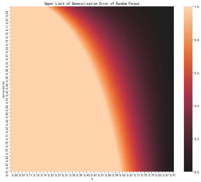
We observe that

1. The stronger the strength, the lower the population error upper bound.
2. The smaller the correlation, the lower the population error upper bound.
3. If the strength is too low, it is very hard for the model to avoid errors.
4. If the correlation is very high, it is still possible to get a decent model if the strength is high.

Random Forest Regressor

Similar to decision trees, random forest can also be used as regressors. The random forest regressor population error is capped by the average population error of trees multiplied by the correlation of trees³.

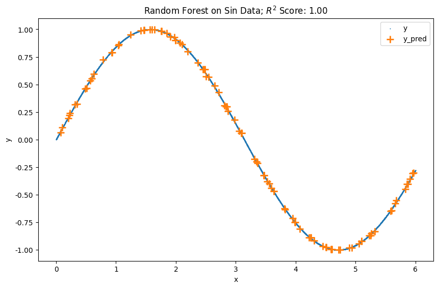
To see how the regressor works with data, we construct an artificial problem. The code can be accessed here .

Sinusoid DataSinusoid Data with NoiseComparing Tow Scenarios

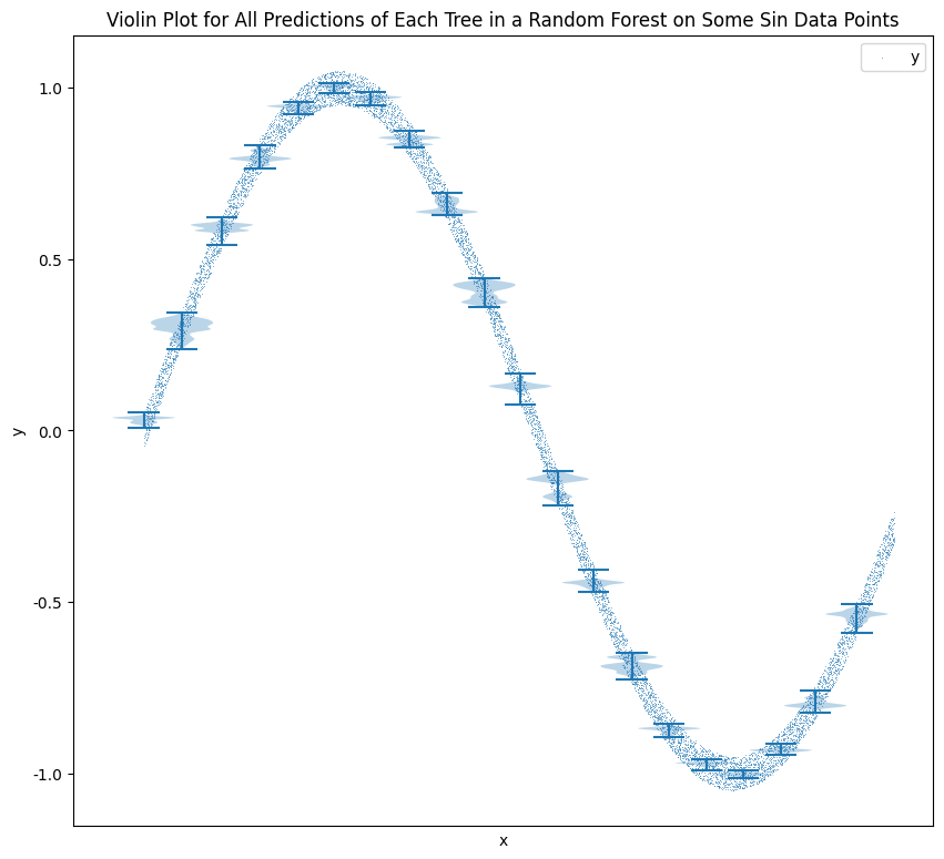
A random forest with 1600 estimators can estimate the following sin data. Note that this is in-sample fitting and prediction to demonstrate the capability of representing sin data.

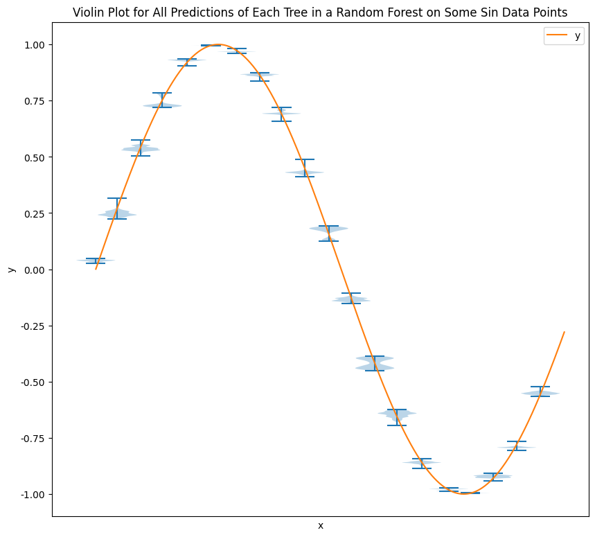
One observation is that not all the trees spit out the same values. We observe some quite dispersed predictions from the trees but the ensemble result is very close to the true values.

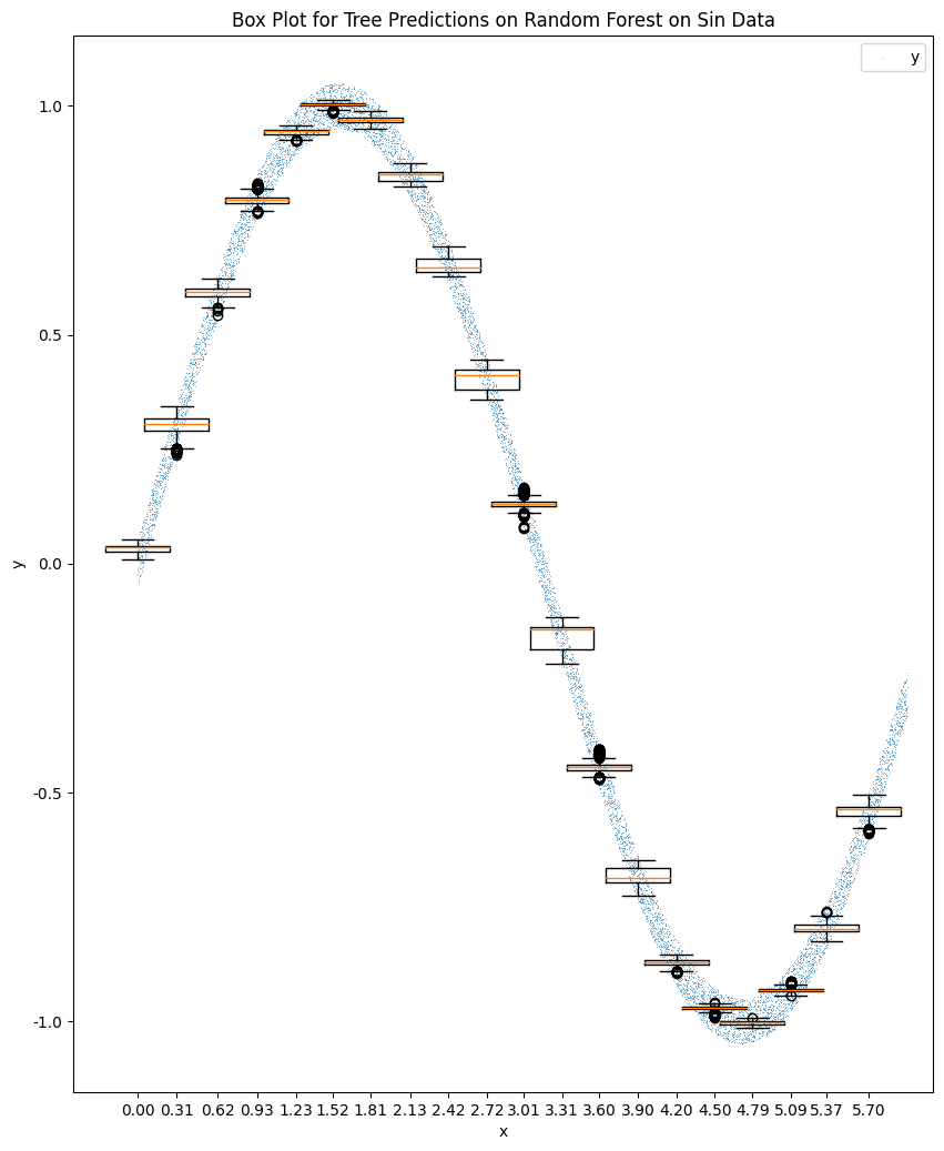
We generate a new dataset by adding some noise to the sin dataset. By adding uniform random noise, we introduce some variance but not much bias in the data. We are cheating a bit here because this kind of data is what random forest is good at.

We train a random forest model with 1300 estimators using this noise data. Note that this is in-sample fitting and prediction to demonstrate the representation capability.

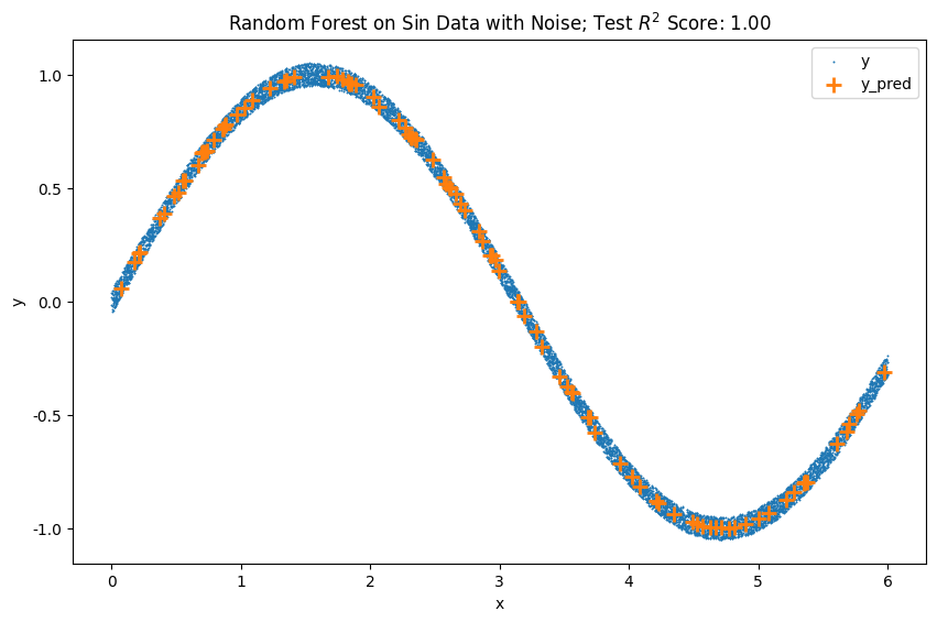
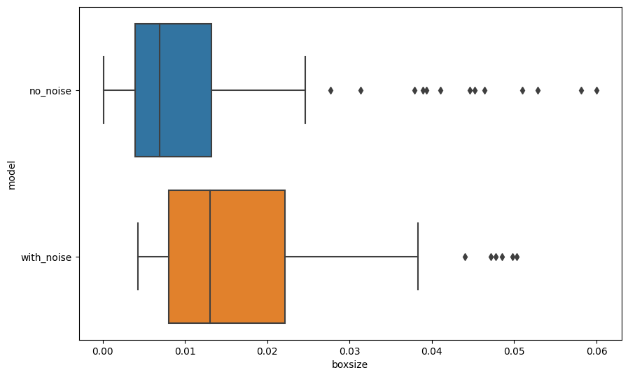
One observation is that not all the trees spit out the same values. The predictions from the trees are sometimes dispersed and not even bell-like, the ensemble result reflects the values of the true sin data. The ensemble results are even located at the center of the noisy data where the true sin values should be. However, we will see that the distribution of the predictions is more dispersed than the model trained without noise (see the tab "Comparing Tow Scenarios").

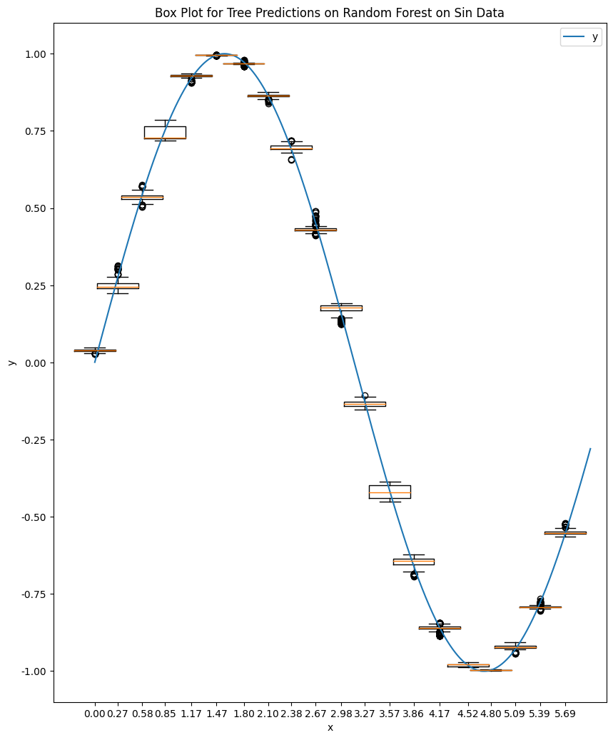
The following two charts show the boxes for the two trainings.

To see the differences between the box sizes for in a more quantitive way, we plot out the box plot of the box sizes for each training.

---

1. Ho TK. Random decision forests. In: Proceedings of 3rd international conference on document analysis and recognition. 1995, pp 278–282 vol.1. ↩

2. Hastie T, Tibshirani R, Friedman J. The elements of statistical learning: Data mining, inference, and prediction. Springer Science & Business Media, 2013. ↩

3. Breiman L. Random forests. Machine learning 2001; 45: 5–32. ↩↩↩↩↩↩↩

4. Bernard S, Heutte L, Adam S. A study of strength and correlation in random forests. In: Advanced intelligent computing theories and applications. Springer Berlin Heidelberg, 2010, pp 186–191. ↩↩

---

Contributors: LM