The Time Delay Embedding Representation¶

The time delay embedding representation of time series data is widely used in deep learning forecasting models¹. This is also called rolling in many time series analyses ².

For simplicity, we only write down the representation for a problem with time series \(y_{1}, \cdots, y_{t}\), and forecasting \(y_{t+1}\). We rewrite the series into a matrix, in an autoregressive way,

\[ \begin{align} \mathbf Y = \begin{bmatrix} y_1 & y_2 & \cdots & y_p &\Big| & {\color{red}y_{p+1}} \\ y_{1+1} & y_{1+2} & \cdots & y_{1+p} &\Big| & {\color{red}y_{1+p+1}} \\ \vdots & \vdots & \ddots & \vdots &\Big| & {\color{red}\vdots} \\ y_{i-p+1} & y_{i-p+2} & \cdots & y_{i} &\Big| & {\color{red}y_{i+1}} \\ \vdots & \vdots & \ddots & \vdots &\Big| & {\color{red}\vdots} \\ y_{t-p+1} & y_{t-p+2} & \cdots & y_{t} &\Big| & {\color{red}y_{t+1}} \\ \end{bmatrix} \end{align} \]

which indicates that we will use everything on the left, a matrix of shape \((t-p+1,p)\), to predict the vector on the right (in red). This is a useful representation when building deep learning models as many of the neural networks require fixed-length inputs.

Taken's Theorem¶

The reason that time delayed embedding representation is useful is that it is a representation of the original time series that preserves the dynamics of the original time series, if any. The math behind it is the Taken's theorem ³.

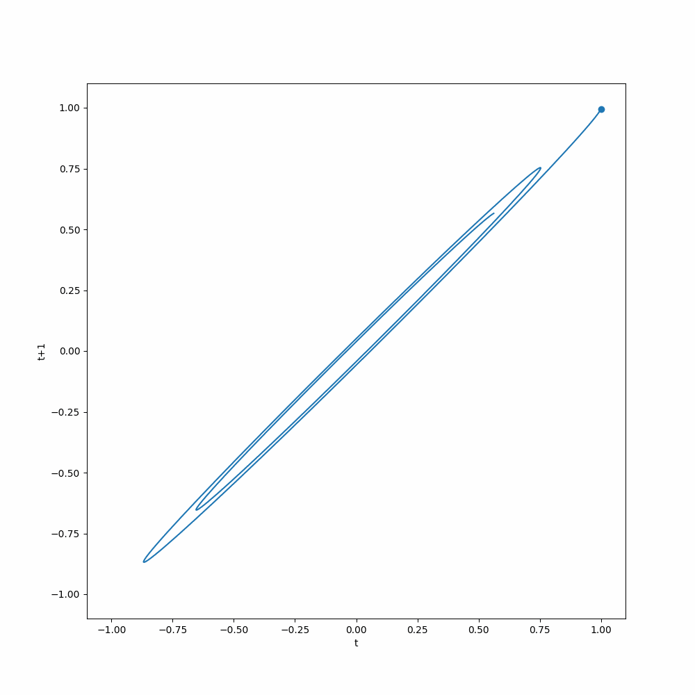
To illustrate the idea, we take our pendulum dataset as an example. The pendulum dataset describes a damped pendulum, for the math and visualizations please refer to the corresponding page. Here we apply the time delay embedding representation to the pendulum dataset by setting both the history length and the target length to 1, so that we can better visualize it.

Animation of Delayed Embedding Code

We plot out the delayed embedding representation of the pendulum dataset. The x-axis is the value of the pendulum angle at time \(t\), and the y-axis is the value of the pendulum angle at time \(t+1\). The animation shows how the delayed embedding representation evolves over time and shows attractor behavior. If a model can capture this dynamics, it can make good predictions.

Delayed Embedding

The notebook for more about the dataset itself is here.

from functools import cached_property
from typing import List, Tuple

import matplotlib as mpl
import matplotlib.animation as animation
import matplotlib.pyplot as plt
import pandas as pd
from ts_dl_utils.datasets.dataset import DataFrameDataset
from ts_dl_utils.datasets.pendulum import Pendulum


ds_de = DataFrameDataset(dataframe=df["theta"][:200], history_length=1, horizon=1)

class DelayedEmbeddingAnimation:
    """Builds an animation for univariate time series
    using delayed embedding.

    ```python
    fig, ax = plt.subplots(figsize=(10, 10))

    dea = DelayedEmbeddingAnimation(dataset=ds_de, fig=fig, ax=ax)
    ani = dea.build(interval=10, save_count=dea.time_steps)
    ani.save("results/pendulum_dataset/delayed_embedding_animation.mp4")
    ```

    :param dataset: a PyTorch dataset, input and target should have only length 1
    :param fig: figure object from matplotlib
    :param ax: axis object from matplotlib
    """
    def __init__(
        self, dataset: DataFrameDataset, fig: mpl.figure.Figure, ax: mpl.axes.Axes
    ):
        self.dataset = dataset
        self.ax = ax
        self.fig = fig

    @cached_property
    def data(self) -> List[Tuple[float, float]]:
        return [(i[0][0], i[1][0]) for i in self.dataset]

    @cached_property
    def x(self):
        return [i[0] for i in self.data]

    @cached_property
    def y(self):
        return [i[1] for i in self.data]

    def data_gen(self):
        for i in self.data:
            yield i

    def animation_init(self) -> mpl.axes.Axes:
        ax.plot(
            self.x,
            self.y,
        )
        ax.set_xlim([-1.1, 1.1])
        ax.set_ylim([-1.1, 1.1])
        ax.set_xlabel("t")
        ax.set_ylabel("t+1")

        return self.ax

    def animation_run(self, data: Tuple[float, float]) -> mpl.axes.Axes:
        x, y = data
        self.ax.scatter(x, y)
        return self.ax

    @cached_property
    def time_steps(self):
        return len(self.data)

    def build(self, interval: int = 10, save_count: int = 10):
        return animation.FuncAnimation(
            self.fig,
            self.animation_run,
            self.data_gen,
            interval=interval,
            init_func=self.animation_init,
            save_count=save_count,
        )


fig, ax = plt.subplots(figsize=(10, 10))

dea = DelayedEmbeddingAnimation(dataset=ds_de, fig=fig, ax=ax)

ani = dea.build(interval=10, save_count=dea.time_steps)

gif_writer = animation.PillowWriter(fps=5, metadata=dict(artist="Lei Ma"), bitrate=100)

ani.save("results/pendulum_dataset/delayed_embedding_animation.gif", writer=gif_writer)
# ani.save("results/pendulum_dataset/delayed_embedding_animation.mp4")

In some advanced deep learning models, delayed embedding plays a crucial role. For example, Large Language Models (LLM) can perform good forecasts by taking in delayed embedding of time series⁴.

Hewamalage H, Ackermann K, Bergmeir C. Forecast evaluation for data scientists: Common pitfalls and best practices. 2022.http://arxiv.org/abs/2203.10716. ↩
Zivot E, Wang J. Modeling financial time series with s-PLUS. Springer New York, 2006 doi:10.1007/978-0-387-32348-0. ↩
Takens F. Detecting strange attractors in turbulence. In: Lecture notes in mathematics. Springer Berlin Heidelberg: Berlin, Heidelberg, 1981, pp 366–381. ↩
Rasul K, Ashok A, Williams AR, Khorasani A, Adamopoulos G, Bhagwatkar R et al. Lag-llama: Towards foundation models for time series forecasting. arXiv [csLG] 2023.http://arxiv.org/abs/2310.08278. ↩

Contributors: LM