Recurrent Neural Networks

In the section Neural Networks, we discussed the feedforward neural network.

Biological Neural Networks

Biological neural networks contain recurrent units. There are theories that employ recurrent networks to explain our memory³.

Recurrent Neural Network Architecture

A recurrent neural network (RNN) can be achieved by including loops in the network, i.e., the output of a unit is fed back to itself. As an example, we show a single unit in the following figure.

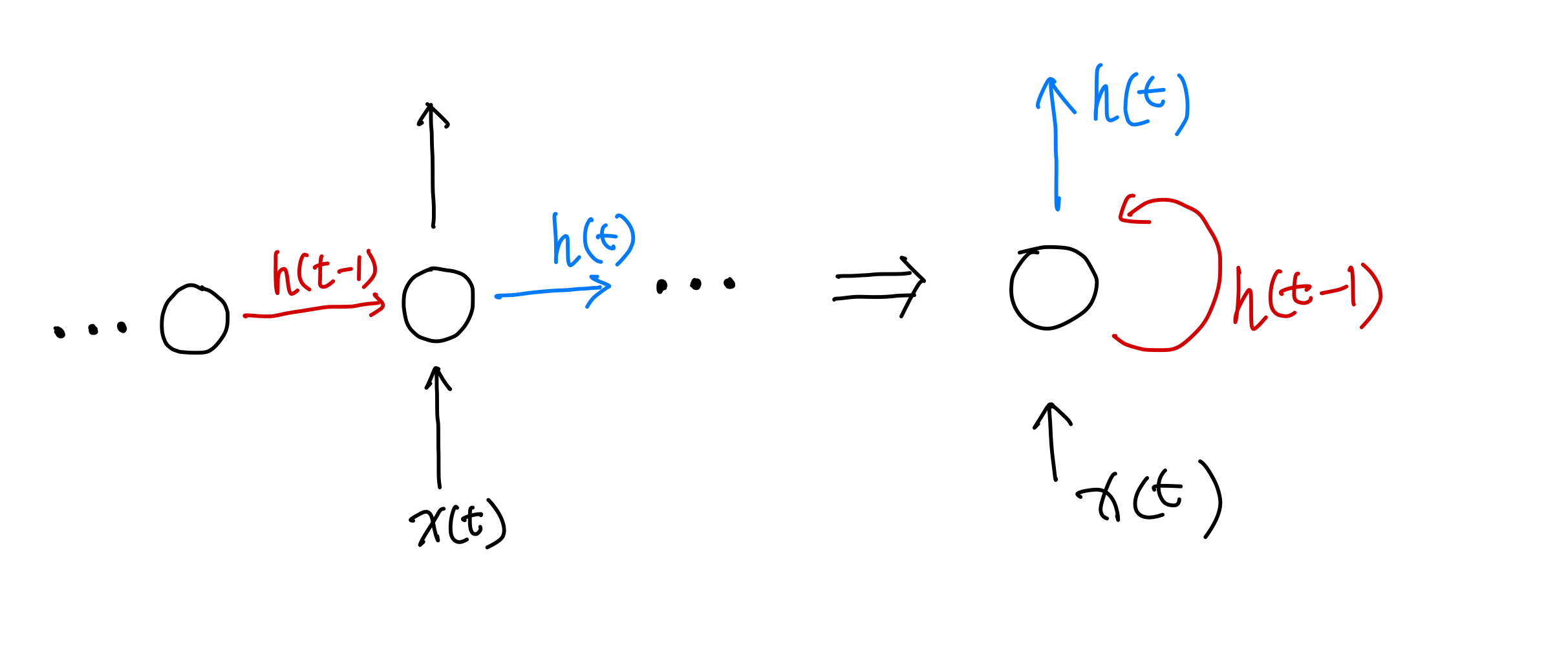
On the left, we have the unfolded (unrolled) RNN, while the representation on the right is the compressed form. A simplified mathematical representation of the RNN is as follows:

\[ \begin{equation} h(t) = f( W_h h(t-1) + W_x x(t) + b) \label{eq-rnn-vanilla} \end{equation} \]

where \(h(t)\) represents the state of the unit at time \(t\), \(x(t)\) is the input at time \(t\).

RNN and First-order Differential Equation

There are different views of the nature of time series data. Many of the time series datasets are generated by physical systems that follow the laws of physics. Mathematicians and physicists already studied and built up the theories of such systems and the framework we are looking into is dynamical systems.

The vanilla RNN described in \(\eqref{eq-rnn-vanilla}\) is quite similar to a first-order differential equation. For simplicity we use RELU for \(f(\cdot)\).

Note that

\[ h(t - 1) = h(t) + \sum_{n=1}^{\infty} \frac{h^{(n)} (t)}{n!} (-1)^n, \]

where \(h^{(n)}(t)\) is the \(n\)th derivative of \(h(t)\). Assuming that it converges and higher order doesn't contribute much, we rewrite \(\eqref{eq-rnn-vanilla}\) as

\[ \begin{equation} \frac{\mathrm d h(t)}{\mathrm d t} = x'(t) + W_h h(t), \label{eq-rnn-1st-order-diff-eq} \end{equation} \]

where

\[ \begin{align} x'(t) =& W_h^{-1} W_x x(t) + b' \\ b' = & W_h^{-1} b. \end{align} \]

We have reduced the RNN formula to a first-order differential equation. Without discussing the details, we know that an exponential component \(e^{W_h t}\) will rise in the solution. The component may explode or shrink.

Based on our intuition of differential equations, such a dynamical system usually just blows up or diminishes for a large number of iterations. It can also be shown explicitly if we write down the backprogation formula where the state in the far past contributes little to the gradient. This is the famous vanishing gradient problem in RNN⁴. One solution to this is to introduce memory in the iterations, e.g., long short-term memory (LSTM) ⁵.

In the basic example of RNN shown above, the output of the hidden state is fed to itself in the next iteration. In theory, the value to feed back to the unit and how the input and output are calculated can be quite different in different setups ¹². In the section Forecasting with RNN, we will show some examples of the different setups.

---

1. Amidi A, Amidi S. CS 230. In: Recurrent Neural Networks Cheatsheet [Internet]. [cited 22 Nov 2023]. Available: https://stanford.edu/~shervine/teaching/cs-230/cheatsheet-recurrent-neural-networks ↩

2. Karpathy A. The Unreasonable Effectiveness of Recurrent Neural Networks. In: Andrej Karpathy blog [Internet]. 2015 [cited 22 Nov 2023]. Available: https://karpathy.github.io/2015/05/21/rnn-effectiveness/ ↩

3. Grossberg S. Recurrent neural networks. Scholarpedia 2013; 8: 1888. ↩

4. Pascanu R, Mikolov T, Bengio Y. On the difficulty of training recurrent neural networks. 2012.http://arxiv.org/abs/1211.5063. ↩

5. Hochreiter S, Schmidhuber J. Long short-term memory. Neural computation 1997; 9: 1735–1780. ↩

---

Contributors: LM