TimeGrad Using Diffusion Model

Rasul et al., (2021) proposed a probabilistic forecasting model using denoising diffusion models.

Autoregressive

Multivariate Forecasting Problem

Given an input sequence \(\mathbf x_{t-K: t}\), we forecast \(\mathbf x_{t+1:t+H}\).

See this section for more Time Series Forecasting Tasks.

Notation

We use \(x^0\) to denote the actual time series. The super script \({}^{0}\) will be used to represent the non-diffused values.

To apply the denoising diffusion model in a multivariate forecasting problem, we define our forecasting task as the following autoregressive problem,

\[ q(\mathbf x^0_{t - K:t} \vert \mathbf x^0_{1:t_0 - 1}) = \Pi_{t=t_0}^T q(\mathbf x^0_t \vert \mathbf x^0_{1:t-1}). \]

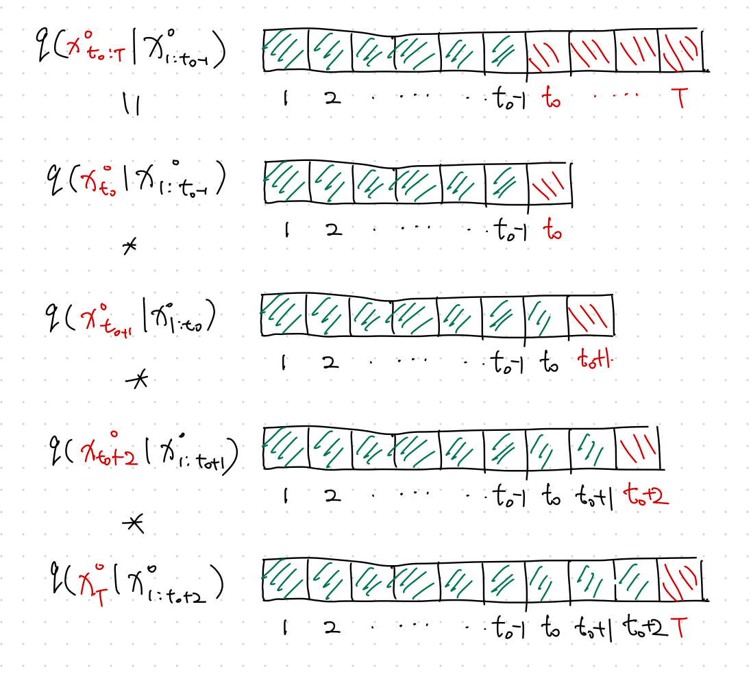
At each time step \(t\), we build a denoising diffusion model.

Time Dynamics

Note that in the denoising diffusion model, we minimize

\[ \operatorname{min}_\theta \mathbb E_{q(\mathbf x^0)} \left[ -\log p_\theta (\mathbf x^0) \right] \]

The above loss becomes that of the denoising model for a single time step. Explicitly,

\[ \operatorname{min}_\theta \mathbb E_{q(\mathbf x^0_t )} \left[ -\log p_\theta (\mathbf x^0_t) \right]. \]

Time dynamics can be easily captured by some RNN. To include the time dynamics, we use the RNN state built using the time series data of the previous time step \(\mathbf h_{t-1}\)¹

\[ \operatorname{min}_\theta \mathbb E_{q(\mathbf x^0_t )} \left[ -\log p_\theta (\mathbf x^0_t \vert \mathbf h_{t-1}) \right]. \]

Apart from the usual time dimension \(t\), the autoregressive denoising diffusion model has another dimension to optimize: the diffusion step \(n\) for each time \(t\).

The loss for each time step \(t\) is¹

\[ \begin{equation} \mathcal L_t = \mathbb E_{\mathbf x^0_t, \epsilon, n} \left[ \lVert \epsilon - \epsilon_\theta ( \sqrt{\bar \alpha_n} \mathbf x^0_t + \sqrt{1-\bar \alpha_n}\epsilon, \mathbf h_{t-1}, n ) \rVert^2 \right]. \label{eq:ddpm-loss} \end{equation} \]

That being said, we just need to minimize \(\mathcal L_t\) for each time step \(t\).

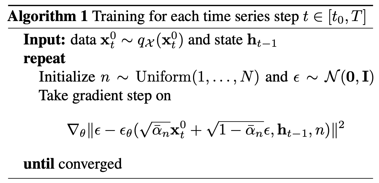
Training Algorithm

The input data is sliced into fixed length time series \(\mathbf x_t^0\). Since Eq \eqref{eq:ddpm-loss} shows that a loss can be calculated for arbitrary \(n\) without depending on any previous diffusion steps \(n-1\), the training can be done by both random sampling in \(\mathbf x_t^0\) and \(n\). See Rasul et al. (2021)¹.

How to Forecast

After training, we obtain the time dynamics encoding \(\mathbf h_T\), with which the denoising steps can be calculated using the reverse process

\[ \mathbf x^{n-1}_{T+1} = \frac{1}{\alpha_n} \left( \mathbf x^n_{T+1} - \frac{\beta_n}{1 - \bar\alpha_n} \epsilon_\theta( \mathbf x^n_{T+1}, \mathbf h_{T}, n ) \right) + \sqrt{\Sigma_\theta} \mathbf z, \]

where \(\mathbf z \sim \mathcal N(\mathbf 0, \mathbf I)\).

For example,

\[ \mathbf x^{0}_{T+1} = \frac{1}{\alpha_1} \left( \mathbf x^1_{T+1} - \frac{\beta_1}{1 - \bar\alpha_1} \epsilon_\theta( \mathbf x^1_{T+1}, \mathbf h_{T}, 1 ) \right) + \sqrt{\Sigma_\theta} \mathbf z. \]

It is Probabilistic

The quantiles is calculated by repeating many times for each forecasted time step¹.

Code

An implementation of the model can be found in the package pytorch-ts ².

---

1. Rasul K, Seward C, Schuster I, Vollgraf R. Autoregressive Denoising Diffusion Models for Multivariate Probabilistic Time Series Forecasting. arXiv [cs.LG]. 2021. Available: http://arxiv.org/abs/2101.12072 ↩↩↩↩

2. Rasul K. PyTorchTS. https://github.com/zalandoresearch/pytorch-ts. ↩

---

Contributors: LM