Neural Networks

Neural networks have been a buzzword for machine learning in recent years. As indicated in the name, artificial neural networks are artificial neurons connected in a network. In this section, we discuss some intuitions and theories of neural networks.

Artificial vs Biological

Neuroscientists also discuss neural networks, or neuronal networks in their research. Those are different concepts from the artificial neural networks we are going to discuss here. In this book, we use the term neural networks to refer to artificial neural networks, unless otherwise specified.

Intuitions

We start with some intuitions of neural networks before discussing the theoretical implications.

What is an Artificial Neuron

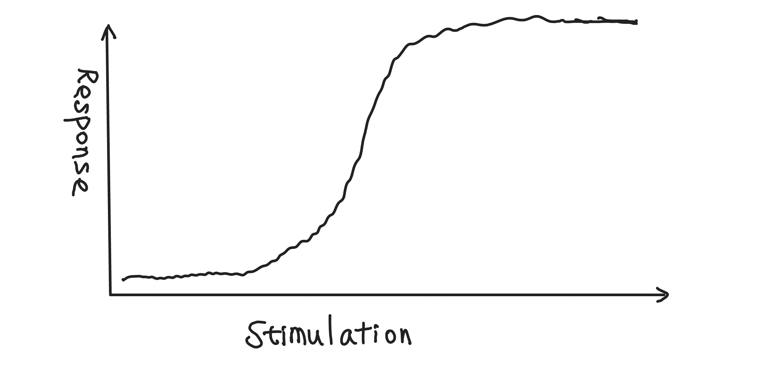
What an artificial neuron does is respond to stimulations. This response could be strong or weak depending on the strength of the stimulations. Here is an example.

Using one simple single neuron, we do not have much to build. It is just the function we observe above. However, by connecting multiple neurons in a network, we could compose complicated functions and generalize the scaler function to multi-dimensional functions.

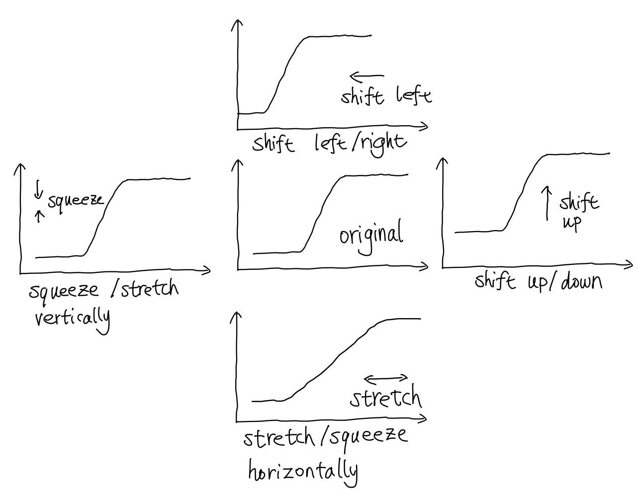
Before we connect this neuron to a network, we study a few transformations first. The response function can be shifted, scaled, or inverted. The following figure shows the effect of these transformations.

Artificial Neural Network

A simple network is a collection of neurons that respond to stimulations, which could come from the responses of other neurons.

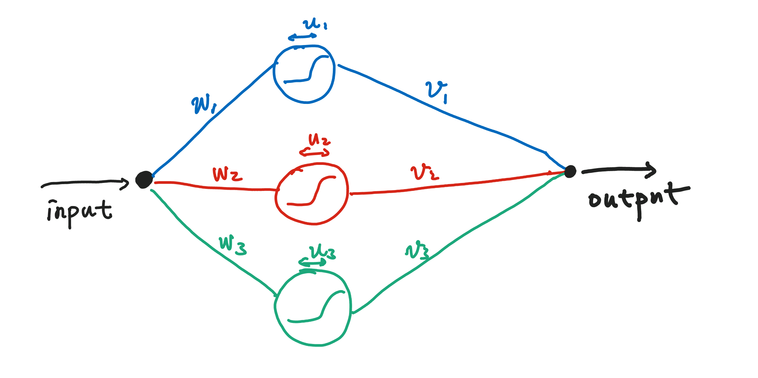
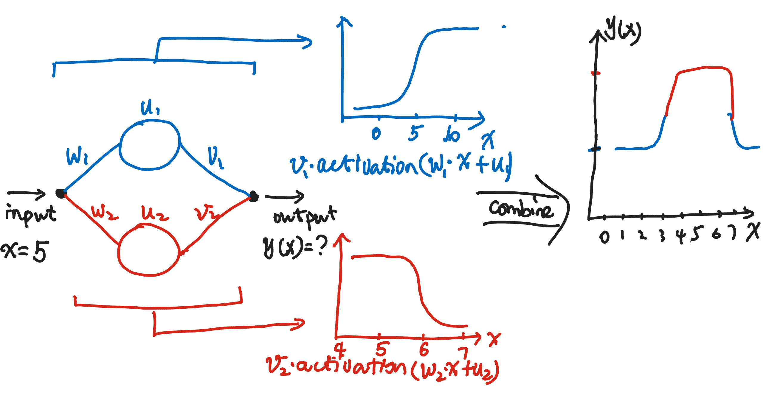
A given input signal is spread onto three different neurons. The neurons respond to this signal separately before being combined with different weights. In the language of math, given input \(x\), output \(y(x)\) is

\[y(x) = \sum_{k=1}^{3} x v_k * \mathrm{activation}( w_k * x + u_k )\]

where \(\mathrm{activation}\) is the activation function, i.e., the response behavior of the neuron. This is a single-layer structure.

\(\mathrm{activation} \to \sigma\)

In the following discussions, we will use \(\sigma\) as a drop in replacement for \(\mathrm{activation}\).

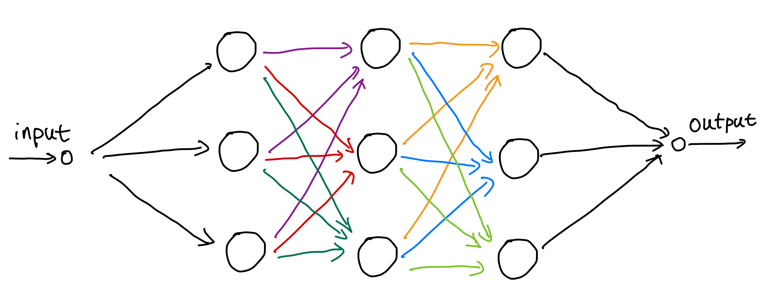
To extend this naive and shallow network, we could

• increase the number of neurons on one layer, i.e., go wider, or
• extend the number of layers, i.e., go deeper, or
• add interactions between neurons, or
• include recurrent connections in the network.

Composition Effects

To build up intuitions of how multiple neurons work together, we take an example of a network with two neurons. We will solve two problems:

1. Find out if a hotel room is hot or cold.
2. Find out if the hotel room is comfortable to stay.

The first task can be solved using o single neuron. Suppose our input to the neuron is the temperature of the room. The output of the neuron is a binary value, 1 for hot and 0 for cold. The following figure shows the response of the neuron.

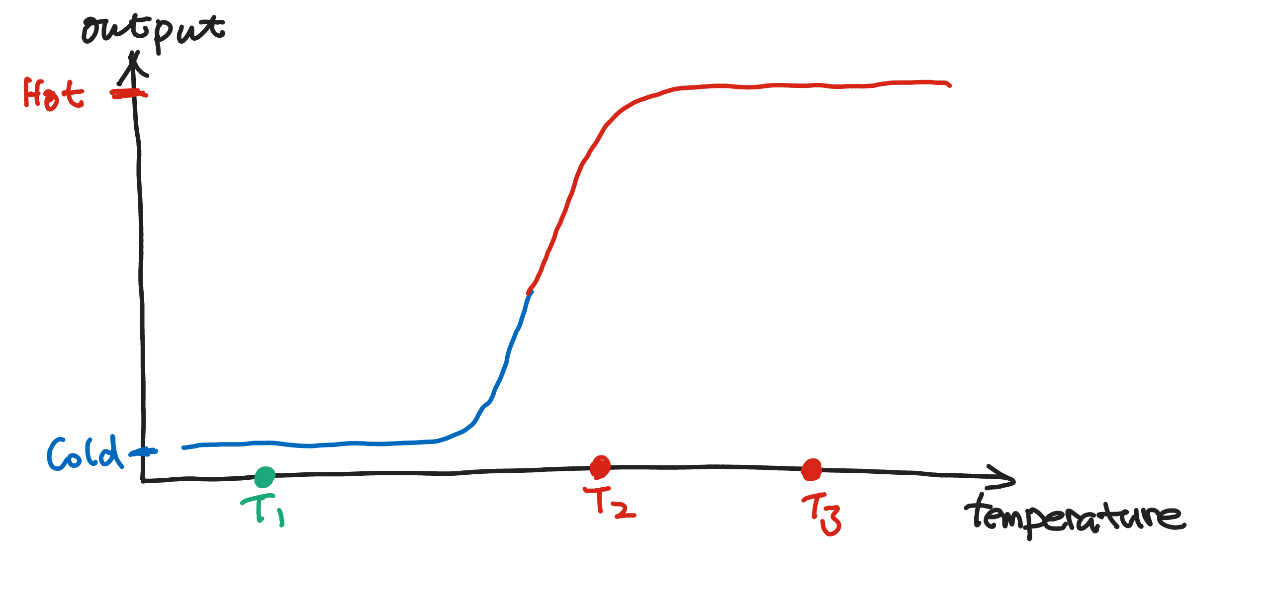
In the figure above, we use red for "hot" and blue for "cold". In this example, the temperature being \(T_1\) means the room is cold, while that being \(T_2\) and \(T_3\) indicate hot rooms.

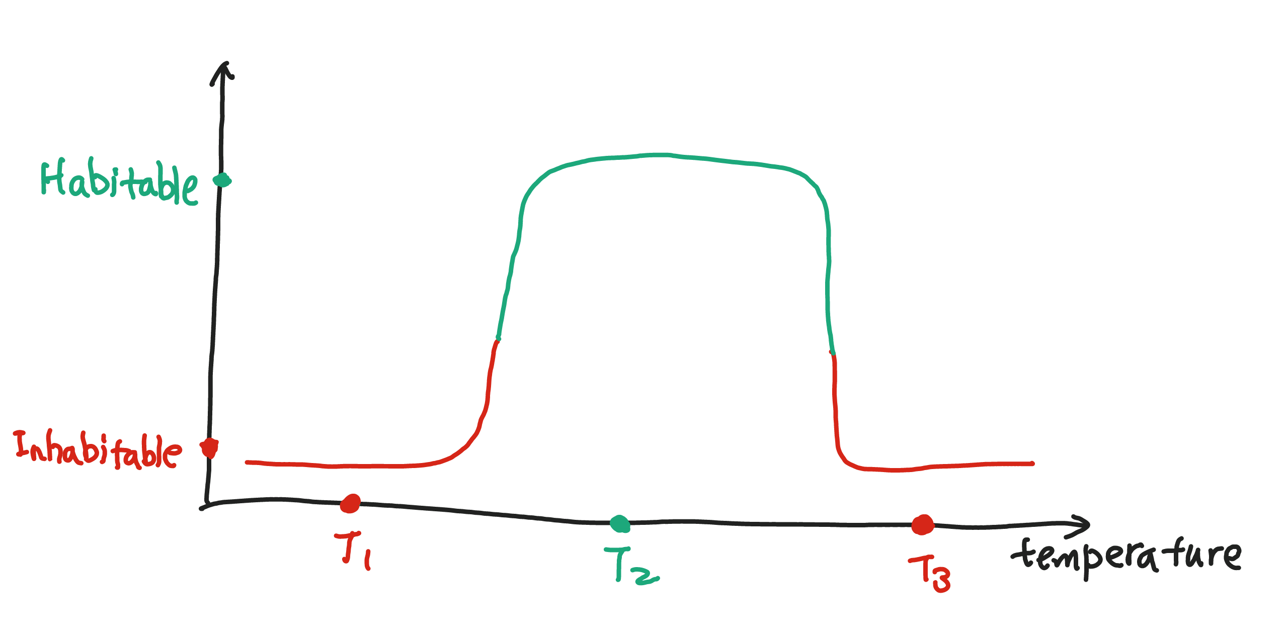
However, moving on the the second problem, such monotonic functions won't work. It is only comfortable to stay in the hotel room if the temperature is neither too high nor too low. Now consider two neurons in a network. One neuron has a monotonic increasing response to the temperature, while the other has a monotonic decreasing response. The following figure shows the combined response of the two neurons. We observe that the combined response is high only when the temperature is in a certain range.

Suppose we have three rooms with temperatures \(T_1\), \(T_2\), \(T_3\) respectively. Only \(T_2\) falls into the region of large output value which corresponds to the habitable temperature.

Mathematical Formulation

The above example can be formulated as $$ f(x) = \sum_k v_k \sigma(w_k x + u_k) $$ where \(\sigma\) is some sort of monotonic activation function.

It is a form of single hidden layer feedforward network. We will discuss this in more detail in the following sections.

These two examples hint that neural networks are good at classification tasks. Neural networks excel at a variety of tasks. Since this book is about time series, we will demonstrate the power of neural networks in time series analysis.

Universal Approximators

Even a single hidden layer feedforward network can approximate any measurable function, regardless of the activation function². In the case of the commonly discussed sigmoid function as an activation function, a neural network for real numbers becomes

\[ \sum_k v_k \sigma(w_k x + u_k) \]

It is a good approximation of continuous functions³.

Kolmogorov's Theorem

Kolmogorov's theorem shows that one can use a finite number of carefully chosen continuous functions to mix up by sums and multiplication with weights to a continuous multivariable function on a compact set⁴.

Neural Networks Can be Complicated

In practice, we observe a lot of problems when the number of neurons grows, e.g., the convergence during the training slows down if we have too many layers in the network (the vanishing gradient problem) ⁵.

Training

We have not yet discussed how to adjust the parameters in a neural network. The process is called training. The most popular method is backpropagation¹.

The reader should understand that a good neural network model is not only about these naive examples but is about many different topics. For example, to solve the vanishing gradient problem, new architectures are proposed, e.g., residual blocks⁶, new optimization techniques were proposed⁷, and theories such as information highway also became the key to the success of deep neural networks⁸.

---

1. Nielsen MA. How the backpropagation algorithm works. In: Neural networks and deep learning [Internet]. [cited 22 Nov 2023]. Available: http://neuralnetworksanddeeplearning.com/chap2.html ↩

2. Hornik K, Stinchcombe M, White H. Multilayer feedforward networks are universal approximators. Neural networks: the official journal of the International Neural Network Society 1989; 2: 359–366. ↩

3. Cybenko G. Approximation by superpositions of a sigmoidal function. Mathematics of Control, Signals, and Systems 1989; 2: 303–314. ↩

4. Hassoun M. Fundamentals of artificial neural networks. The MIT Press, Massachusetts Institute of Technology, 2021https://mitpress.mit.edu/9780262514675/fundamentals-of-artificial-neural-networks/. ↩

5. Hochreiter S, Bengio Y, Frasconi P, Schmidhuber J. Gradient flow in recurrent nets: The difficulty of learning long-term dependencies. In: Kremer SC, Kolen JF (eds). A field guide to dynamical recurrent neural networks. IEEE Press, 2001. ↩

6. He K, Zhang X, Ren S, Sun J. Deep residual learning for image recognition. 2015.http://arxiv.org/abs/1512.03385. ↩

7. Huang G, Sun Y, Liu Z, Sedra D, Weinberger K. Deep networks with stochastic depth. 2016.http://arxiv.org/abs/1603.09382. ↩

8. Srivastava RK, Greff K, Schmidhuber J. Highway networks. 2015.http://arxiv.org/abs/1505.00387. ↩

---

Contributors: LM