f-GAN

The essence of GAN is comparing the generated distribution \(p_G\) and the data distribution \(p_\text{data}\). The vanilla GAN considers the Jensen-Shannon divergence \(\operatorname{D}_\text{JS}(p_\text{data}\Vert p_{G})\). The discriminator \({\color{green}D}\) serves the purpose of forcing this divergence to be small.

Why do we need the discriminator?

If the JS divergence is an objective, why do we need the discriminator? Even in f-GAN we need a functional to approximate the f-divergence. This functional we choose works like the discriminator of GAN.

There exists a more generic form of JS divergence, which is called f-divergence¹. f-GAN obtains the model by estimating the f-divergence between the data distribution and the generated distribution².

Variational Divergence Minimization

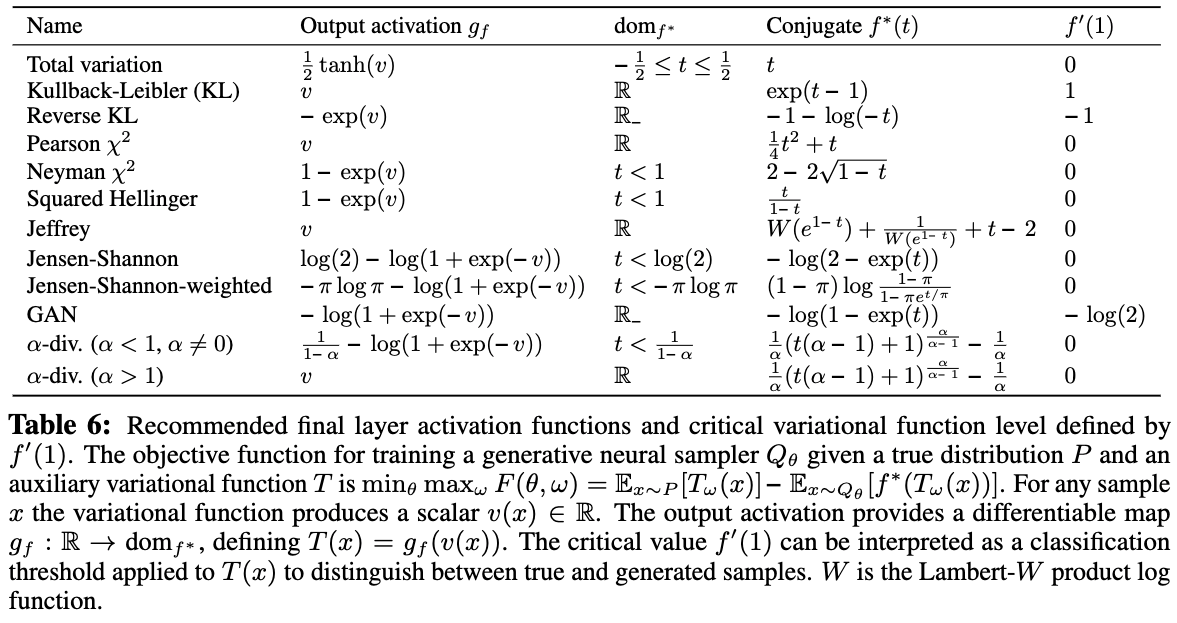
The Variational Divergence Minimization (VDM) extends the variational estimation of f-divergence². VDM searches for the saddle point of an objective \(F({\color{red}\theta}, {\color{blue}\omega})\), i.e., min w.r.t. \(\theta\) and max w.r.t \({\color{blue}\omega}\), where \({\color{red}\theta}\) is the parameter set of the generator \({\color{red}Q_\theta}\), and \({\color{blue}\omega}\) is the parameter set of the variational approximation to estimate f-divergence, \({\color{blue}T_\omega}\).

The objective \(F({\color{red}\theta}, {\color{blue}\omega})\) is related to the choice of \(f\) in f-divergence and the variational functional \({\color{blue}T}\),

\[ \begin{align} & F(\theta, \omega)\\ =& \mathbb E_{x\sim p_\text{data}} \left[ {\color{blue}T_\omega}(x) \right] - \mathbb E_{x\sim {\color{red}Q_\theta} } \left[ f^*({\color{blue}T_\omega}(x)) \right] \\ =& \mathbb E_{x\sim p_\text{data}} \left[ g_f(V_{\color{blue}\omega}(x)) \right] - \mathbb E_{x\sim {\color{red}Q_\theta} } \left[ f^*(g_f(V_{\color{blue}\omega}(x))) \right]. \end{align} \]

In the above objective,

• \(f^*\) is the Legendre–Fenchel transformation of \(f\), i.e., \(f^*(t) = \operatorname{sup}_{u\in \mathrm{dom}_f}\left\{ ut - f(u) \right\}\).

\(T\)

The function \(T\) is used to estimate the lower bound of f-divergence².

Choice of \(g_f\) and \(V\)

Nowozin et al provided a table for \(g_f\) and \(V\)².

We estimate

• \(\mathbb E_{x\sim p_\text{data}}\) by sampling from the mini-batch, and
• \(\mathbb E_{x\sim {\color{red}Q_\theta} }\) by sampling from the generator.

Reduce to GAN

The VDM loss can be reduced to the loss of GAN by setting²

\[ \begin{align} \log {\color{green}D_\omega} =& g_f(V_{\color{blue}\omega}(x)) \\ \log \left( 1 - {\color{green}D_\omega} \right) =& -f^*\left( g_f(V_{\color{blue}\omega}(x)) \right). \end{align} \]

It is straightforward to validate that the following result is a solution to the above set of equations,

\[ g_f(V) = \log \frac{1}{1 + e^{-V}}. \]

Code

• minlee077/f-GAN-pytorch
• shayneobrien/generative-models

---

1. Contributors to Wikimedia projects. F-divergence. In: Wikipedia [Internet]. 17 Jul 2021 [cited 6 Sep 2021]. Available: https://en.wikipedia.org/wiki/F-divergence#Instances_of_f-divergences ↩

2. Nowozin S, Cseke B, Tomioka R. f-GAN: Training Generative Neural Samplers using Variational Divergence Minimization. arXiv [stat.ML]. 2016. Available: http://arxiv.org/abs/1606.00709 ↩↩↩↩↩

3. Contributors to Wikimedia projects. Convex conjugate. In: Wikipedia [Internet]. 20 Feb 2021 [cited 7 Sep 2021]. Available: https://en.wikipedia.org/wiki/Convex_conjugate ↩

---

Contributors: LM