Forecasting with RNN

Jupyter Notebook Available

We have a notebook for this section which includes all the code used in this section.

Introduction to Neural Networks

We explain the theories of neural networks in this section. Please read it first if you are not familiar with neural networks.

In section Recurrent Neural Network we discussed the basics of RNN. In this section, we will build an RNN model to forecast our pendulum time series data.

RNN Model

RNN Model Description RNN Model Code

We build an RNN model with an input size of 96, a hidden size of 64 and one single RNN block. We use L1 loss in the trainings.

from typing import Dict

import dataclasses

from torch.utils.data import Dataset, DataLoader
from torch import nn
import torch


@dataclasses.dataclass
class TSRNNParams:
    """A dataclass to be served as our parameters for the model.

    :param hidden_size: number of dimensions in the hidden state
    :param input_size: input dim
    :param num_layers: number of units stacked
    """

    input_size: int
    hidden_size: int
    num_layers: int = 1


class TSRNN(nn.Module):
    """RNN for univaraite time series modeling.

    :param history_length: the length of the input history.
    :param horizon: the number of steps to be forecasted.
    :param rnn_params: the parameters for the RNN network.
    """

    def __init__(self, history_length: int, horizon: int, rnn_params: TSRNNParams):
        super().__init__()
        self.rnn_params = rnn_params
        self.history_length = history_length
        self.horizon = horizon

        self.regulate_input = nn.Linear(
            self.history_length, self.rnn_params.input_size
        )

        self.rnn = nn.RNN(
            input_size=self.rnn_params.input_size,
            hidden_size=self.rnn_params.hidden_size,
            num_layers=self.rnn_params.num_layers,
            batch_first=True
        )

        self.regulate_output = nn.Linear(
            self.rnn_params.hidden_size, self.horizon
        )

    @property
    def rnn_config(self) -> Dict:
        return dataclasses.asdict(self.rnn_params)

    def forward(self, x: torch.Tensor) -> torch.Tensor:
        x = self.regulate_input(x)
        x, _ = self.rnn(x)

        return self.regulate_output(x)

One Step Forecasting

Similar to Forecasting with Feedforward Neural Networks, we take 100 time steps as the input history and forecast 1 time step into the future, but with a gap of 10 time steps.

Training

The details for model training can be found in this notebook. We will skip the details but show the loss curve here.

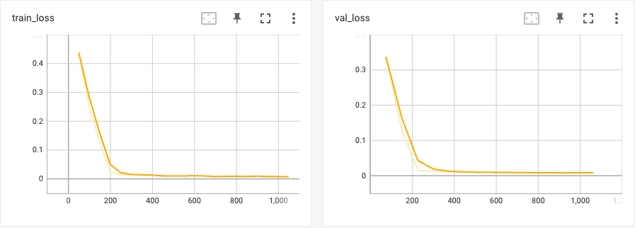
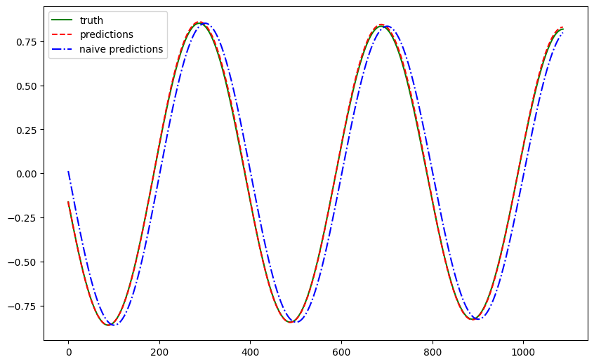
With just a few seconds of training, our RNN model can capture the pattern of the pendulum time series data.

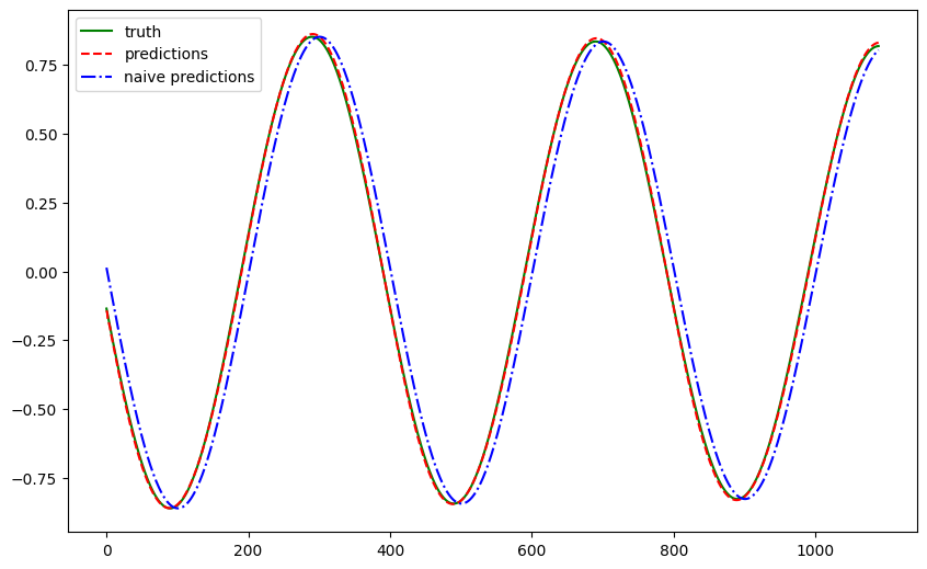
The metrics are listed in the following table.

Metric	RNN	Naive
Mean Absolute Error	0.007229	0.092666
Mean Squared Error	0.000074	0.010553
Symmetric Mean Absolute Percentage Error	0.037245	0.376550

Multi-Horizon Forecasting

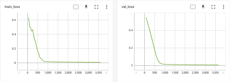
We also trained the same model to forecast 3 steps into the future and also with a gap of 10 time steps.

Training

The details for model training can be found in this notebook. We will skip the details but show the loss curve here.

Visualizing a few examples of the forecasts, it looks reasonable in many cases.

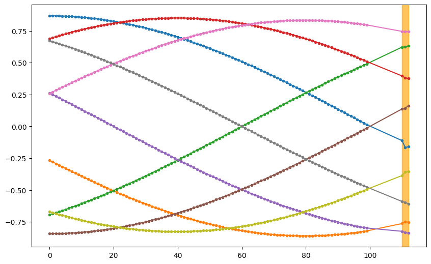
Similar to the single step forecast, we visualize a specific time step in the forecasts and comparing it to the ground truths. Here we choose to visualize the second time step in the forecasts.

The metrics are listed in the following table.

Metric	RNN	Naive
Mean Absolute Error	0.006714	0.109485
Mean Squared Error	0.000069	0.014723
Symmetric Mean Absolute Percentage Error	0.032914	0.423563

---

Contributors: LM