VAR
VAR(1)
VAR(1) is similar to AR(1) but models time series with interactions between the series. For example, a two-dimensional VAR(1) model is
A more compact form is
Stability of VAR
For VAR(1), our series blows up when the max eigenvalue of the matrix \(\boldsymbol \phi_1\) is large than 11. Otherwise, we get stable series.
In the following examples, we denote the largest eigenvalue of \(\boldsymbol \phi_1\) as \(\lambda_0\).
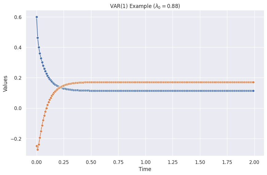
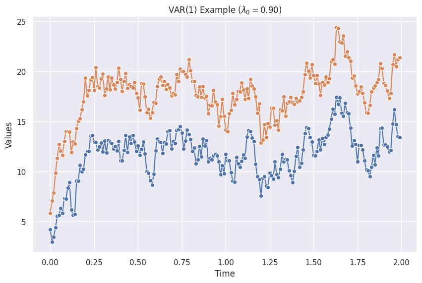
The figure is created using the code from the "Python Code" tab, and the following parameters.
var_params_stable = VAR1ModelParams(
    delta_t = 0.01,
    phi0 = np.array([0.1, 0.1]),
    phi1 = np.array([
        [0.5, -0.25],
        [-0.35, 0.45+0.2]
    ]),
    epsilon = ConstantEpsilon(epsilon=np.array([0,0])),
    initial_state = np.array([1, 0])
)

var1_visualize(var_params=var_params_stable)
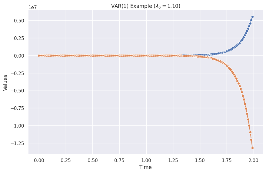
The figure is created using the code from the "Python Code" tab, and the following parameters.
var_params_unstable = VAR1ModelParams(
    delta_t = 0.01,
    phi0 = np.array([0.1, 0.1]),
    phi1 = np.array([
        [0.5, -0.25],
        [-0.35, 0.45+0.5]
    ]),
    epsilon = ConstantEpsilon(epsilon=np.array([0,0])),
    initial_state = np.array([1, 0])
)

var1_visualize(var_params=var_params_unstable)
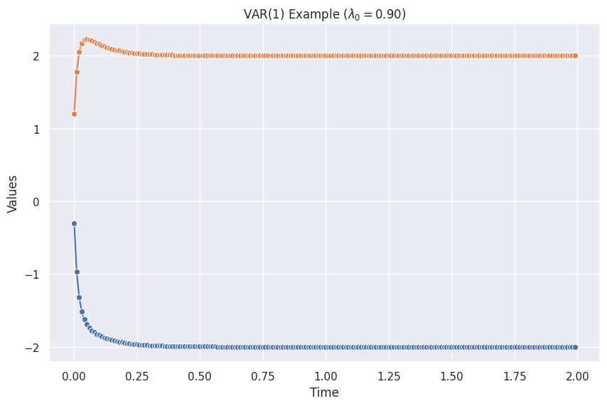
The figure is created using the code from the "Python Code" tab, and the following parameters.
var_params_no_noise = VAR1ModelParams(
    delta_t = 0.01,
    phi0 = np.array([-1, 1]),
    phi1 = np.array([
        [0.7, 0.2],
        [0.2, 0.7]
    ]),
    epsilon = ConstantEpsilon(epsilon=np.array([0,0])),
    initial_state = np.array([1, 0])
)

var1_visualize(var_params=var_params_no_noise)
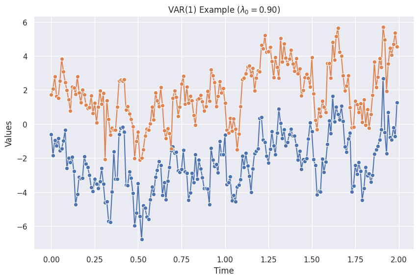
The figure is created using the code from the "Python Code" tab, and the following parameters.
var_params_zero_mean_noise = VAR1ModelParams(
    delta_t = 0.01,
    phi0 = np.array([-1, 1]),
    phi1 = np.array([
        [0.7, 0.2],
        [0.2, 0.7]
    ]),
    epsilon = MultiGaussianNoise(mu=np.array([0, 0]), cov=np.array([[1, 0.5],[0.5, 1]])),
    initial_state = np.array([1, 0])
)

var1_visualize(var_params=var_params_zero_mean_noise)
The figure is created using the code from the "Python Code" tab, and the following parameters.
var_params_nonzero_mean_noise = VAR1ModelParams(
    delta_t = 0.01,
    phi0 = np.array([-1, 1]),
    phi1 = np.array([
        [0.7, 0.2],
        [0.2, 0.7]
    ]),
    epsilon = MultiGaussianNoise(mu=np.array([1, 2]), cov=np.array([[1, 0.5],[0.5, 1]])),
    initial_state = np.array([1, 0])
)

var1_visualize(var_params=var_params_nonzero_mean_noise)
import copy
from dataclasses import dataclass
from typing import Iterator
import numpy as np

class MultiGaussianNoise:
"""A multivariate Gaussian noise

:param mu: means of the variables
:param cov: covariance of the variables
:param seed: seed of the random number generator for reproducibility
"""

def __init__(self, mu: np.ndarray, cov: np.ndarray, seed: Optional[float] = None):
    self.mu = mu
    self.cov = cov
    self.rng = np.random.default_rng(seed=seed)

def __next__(self) -> np.ndarray:
    return self.rng.multivariate_normal(self.mu, self.cov)

class ConstantEpsilon:
"""Constant noise

:param epsilon: the constant value to be returned
"""
def __init__(self, epsilon=0):
    self.epsilon = epsilon

def __next__(self):
    return self.epsilon


@dataclass(frozen=True)
class VAR1ModelParams:
    """Parameters of our VAR model,

    :param delta_t: step size of time in each iteration
    :param phi0: pho_0 in the AR model
    :param phi1: pho_1 in the AR model
    :param epsilon: noise iterator, e.g., Gaussian noise
    :param initial_state: a dictionary of the initial state, e.g., `{"s": 1}`
    """

    delta_t: float
    phi0: np.ndarray
    phi1: np.ndarray
    epsilon: Iterator
    initial_state: np.ndarray


class VAR1Stepper:
    """Calculate the next values using VAR(1) model.

    :param model_params: the parameters of the VAR(1) model, e.g.,
        [`VAR1ModelParams`][eerily.data.generators.var.VAR1ModelParams]
    """

    def __init__(self, model_params):
        self.model_params = model_params
        self.current_state = copy.deepcopy(self.model_params.initial_state)

    def __iter__(self):
        return self

    def __next__(self):

        epsilon = next(self.model_params.epsilon)
        phi0 = self.model_params.phi0
        phi1 = self.model_params.phi1

        self.current_state = phi0 + np.matmul(phi1, self.current_state) + epsilon

        return copy.deepcopy(self.current_state)


class Factory:
    """A generator that creates the data points based on the stepper."""
    def __init__(self):
        pass

    def __call__(self, stepper, length):
        i = 0
        while i < length:
            yield next(stepper)
            i += 1
We create a function to visualize the series.
def var1_visualize(var_params):
    phi1_eig_max = max(np.linalg.eig(var_params.phi1)[0])

    var1_stepper = VAR1Stepper(model_params=var_params)

    length = 200
    fact = Factory()
    history = list(fact(var1_stepper, length=length))

    df = pd.DataFrame(history, columns=["s1", "s2"])
    print(df.head())

    fig, ax = plt.subplots(figsize=(10, 6.18))

    sns.lineplot(
        x=np.linspace(0, length-1, length) * var_params.delta_t,
        y=df.s1,
        ax=ax,
        marker="o",
    )

    sns.lineplot(
        x=np.linspace(0, length-1, length) * var_params.delta_t,
        y=df.s2,
        ax=ax,
        marker="o",
    )

    ax.set_title(f"VAR(1) Example ($\lambda_0={phi1_eig_max:0.2f}$)")
    ax.set_xlabel("Time")
    ax.set_ylabel("Values")
-
Zivot E, Wang J. Modeling Financial Time Series with S-PLUS®. Springer New York; 2006. doi:10.1007/978-0-387-32348-0 ↩