Box-Cox Transformation
In one minute
Real series are often non-stationary, with a variance that changes with the level. The Box-Cox transformation, a family of transforms indexed by λ (λ = 0 is the log), reduces this; the air passenger data shows it in action. It doesn't always produce perfectly stationary data.
Read first: Time Series Analysis
Many time series models require stationary data. However, real-world time series data may be non-stationary and heteroscedastic1. Box-cox transformation is useful when reducing the non-stationarity and heteroscedasticity.
Rob J Hyndman and George Athanasopoulos's famous textbook FPP2 provides some nice examples of box-cox transformations.
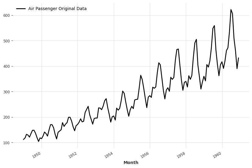
To see Box-Cox transformation in action, we show an example using the air passenger dataset.
The air passenger dataset is a monthly dataset. We can observe the trend and varying variance simply by eyes.
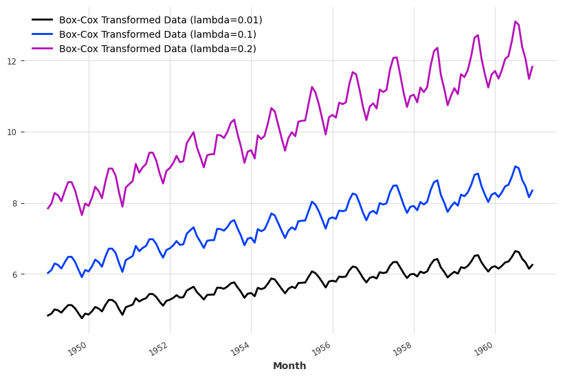
Applying Box-Cox transformations with different lambdas leads to different results shown below. Drag the \(\lambda\) slider to transform the series yourself: \(\lambda = 1\) only shifts the data, \(\lambda = 0\) is the log transform. The lower panel shows the rolling 12-month standard deviation of the transformed series divided by its average, so a flat line at 1 means the variance no longer grows with the level.
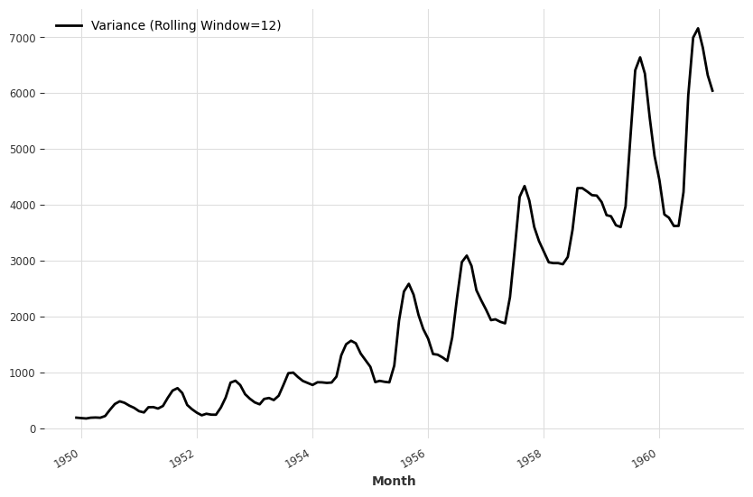
To check the variance, we plot out the variance rolling on a 12-month window.
Box-Cox transformation with \(\lambda =0.1\) reduces the variability in variance.
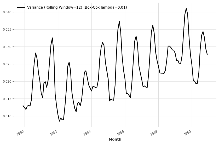
Box-Cox May not Always Reach Perfect Stationary Data
Box-Cox transformation is a simple transformation that helps us reduce the non-stationarity and heteroscedasticy. However, we may not always be able to convert the dataset to stationary and homoscedastic data. This can be observed by performing checks using tools such as stationarity_tests in Darts.
-
Homoscedasticity and heteroscedasticity. (2023, June 2). In Wikipedia. https://en.wikipedia.org/wiki/Homoscedasticity_and_heteroscedasticity ↩