Naive Forecasts¶

In some sense, time series forecasting is easy, if we have low expectations. From a dynamical system point of view, our future is usually not too different from our current state.

Last Observation¶

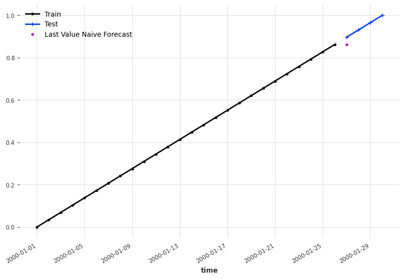
Assuming our time series is not changing dramatically, we can take our last observation as our forecast.

Example: Last Observation as Forecast

Assuming we have the simplest dynamical system,

\[ \frac{\mathrm d y(t)}{\mathrm dt} = f(y, t, \theta), \]

where \(y(t)\) is the time series generator function, \(t\) is time, \(\theta\) is some parameters defining the function \(f\).

For example,

\[ \frac{\mathrm d y(t)}{\mathrm dt} = t \]

is a linear growing time series.

We would imagine, it won't be too crazy if we just take the last observed value as our forecast.

Naive Last Value Forecasts Code

Naive Last Value Forecasts

import matplotlib.pyplot as plt

from darts.utils.timeseries_generation import linear_timeseries

ts = linear_timeseries(length=30)
ts.plot(marker=".")

ts_train, ts_test = ts.split_before(0.9)
ts_train.plot(marker=".", label="Train")
ts_test.plot(marker="+", label="Test")

ts_last_value_naive_forecast = ts_train.shift(1)[-1]

fig, ax = plt.subplots(figsize=(10, 6.18))
ts_train.plot(marker=".", label="Train", ax=ax)
ts_test.plot(marker="+", label="Test", ax=ax)
ts_last_value_naive_forecast.plot(marker=".", label="Last Value Naive Forecast")

There are also slightly more complicated naive forecasting methods.

Mean Forecast¶

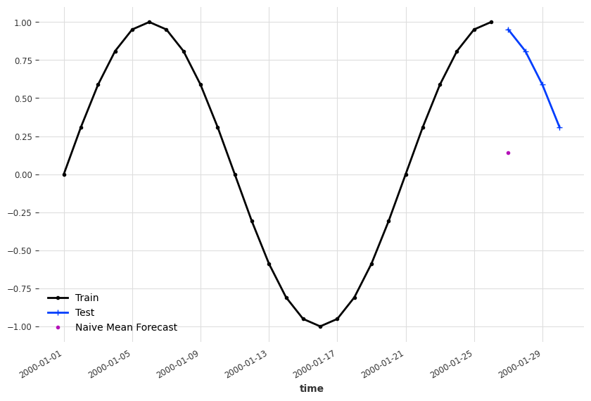
In some bounded time series, the mean of the past values is also a good naive candidate¹.

Example: Naive Mean Forecast

Naive Mean Forecast Code

import matplotlib.pyplot as plt

from darts.utils.timeseries_generation import sine_timeseries
from darts.models.forecasting.baselines import NaiveMean

ts_sin = sine_timeseries(length=30, value_frequency=0.05)

ts_sin.plot(marker=".")


ts_sin_train, ts_sin_test = ts_sin.split_before(0.9)

ts_sin_train.plot(marker=".", label="Train")
ts_sin_test.plot(marker="+", label="Test")


naive_mean_model = NaiveMean()
naive_mean_model.fit(ts_sin_train)
ts_mean_naive_forecast = naive_mean_model.predict(1)

fig, ax = plt.subplots(figsize=(10, 6.18))
ts_sin_train.plot(marker=".", label="Train", ax=ax)
ts_sin_test.plot(marker="+", label="Test", ax=ax)
ts_mean_naive_forecast.plot(marker=".", label="Naive Mean Forecast")

Simple Exponential Smoothing¶

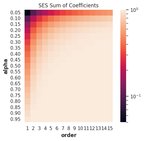
Simple Exponential Smoothing (SES) is a naive smoothing method to account for the historical values of a time series when forecasting. The expanded form of SES is¹

\[ y(t) = \alpha ( y(t-1) + (1-\alpha) y(t-2) + (1-\alpha)^2 y(t-3) + \cdots ) \]

Truncated SES is Biased

Naively speaking, if history is constant, we have to forecast the same constant. For example, if we have \(y(t) = y(t_0)\), the smoothing

\[ y(t) = \alpha (1 + (1-\alpha) + \cdots) y(t_0) \]

should equal to \(y(t_0)\), i.e.,

\[ \alpha (1 + (1-\alpha) + \cdots) = 1. \]

The series indeed sums up to \(1/\alpha\) when \(n\to\infty\) since

\[ \sum_{n=0}^\infty (1-\alpha) = \frac{1}{\alpha}. \]

However, if we truncate the series to finite values, we will have

\[ \sum_{n=0}^N (1-\alpha) \leq \frac{1}{\alpha}. \]

Then our naive forecast for constant series is

\[ y(t) = \alpha \sum_{n=0}^N (1-\alpha) y(t_0) \leq y(t_0), \]

when \(y(t_0)\) is positive.

As an intuition, we plot out the sum of the coefficients for different orders and \(\alpha\)s.

SES Coefficients Code

from itertools import product
import pandas as pd
import seaborn as sns; sns.set()
from matplotlib.colors import LogNorm

def ses_coefficients(alpha, order):
    return (
        np.power(
                np.ones(int(order)) * (1-alpha), np.arange((order))
            ) * alpha
    )

alphas = np.linspace(0.05, 0.95, 19)
orders = list(range(1, 16))

# Create dataframes for visualizations
df_ses_coefficients = pd.DataFrame(
    [[alpha, order] for alpha, order in product(alphas, orders)],
    columns=["alpha", "order"]
)
df_ses_coefficients["ses_coefficients_sum"] = df_ses_coefficients.apply(
    lambda x: ses_coefficients(x["alpha"], x["order"]).sum(), axis=1
)

# Visualization
g = sns.heatmap(
    data=df_ses_coefficients.pivot(
        "alpha", "order", "ses_coefficients_sum"
    ),
    square=True, norm=LogNorm(),
    fmt="0.2g",
    yticklabels=[f"{i:0.2f}" for i in alphas],
)

g.set_title("SES Sum of Coefficients");

Holt-Winters' Exponential Smoothing

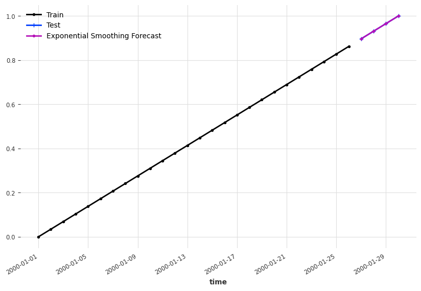
In applications, the Holt-Winters' exponential smoothing is more practical¹²³.

We created some demo time series and apply the Holt-Winters' exponential smoothing. To build see where exponential smoothing works, we forecast at different dates.

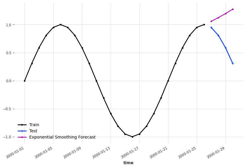
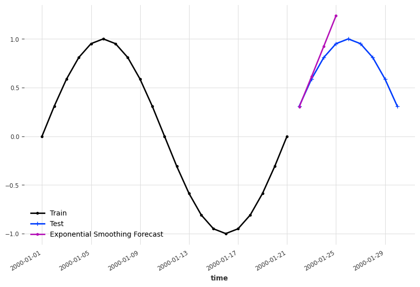
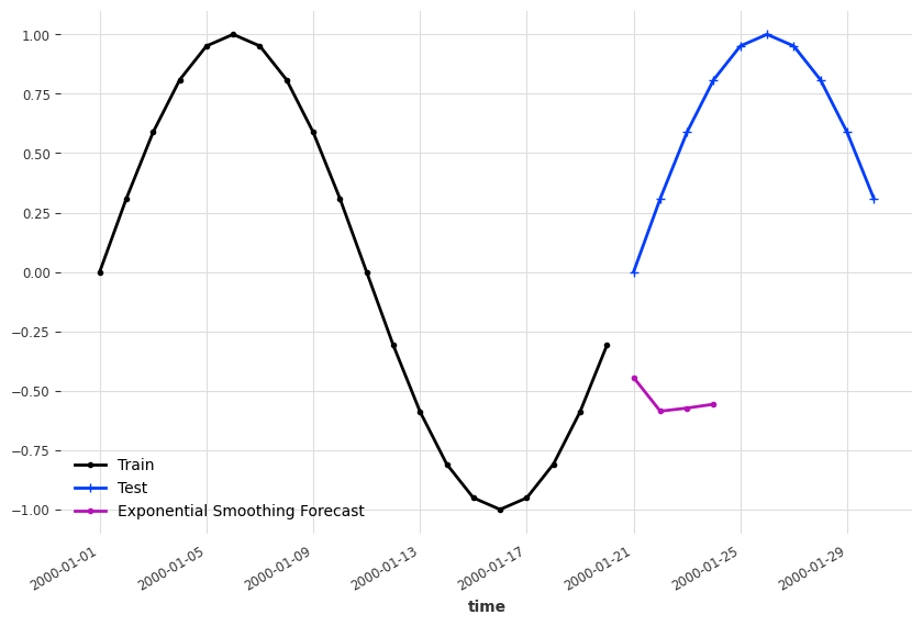
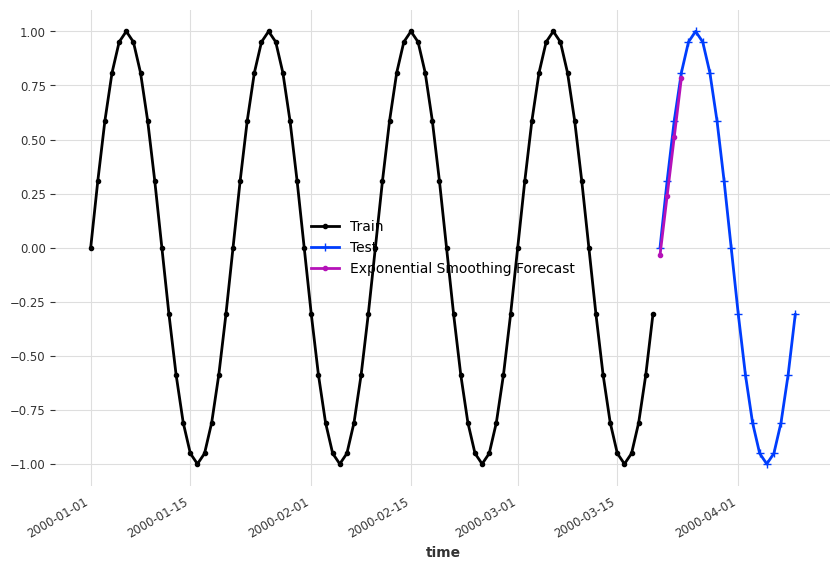
Linear Example Sine Example 1 Sine Example 2 Sine Example 3 Sine Example 3, Longer History Code

import matplotlib.pyplot as plt

from darts.utils.timeseries_generation import sine_timeseries
from darts.models.forecasting.baselines import NaiveMean

ts_sin = sine_timeseries(length=30, value_frequency=0.05)

ts_sin.plot(marker=".")

ts_sin_train, ts_sin_test = ts_sin.split_before(0.7)

es_model = ExponentialSmoothing()

es_model.fit(ts_sin_train)
es_model_sin_forecast = es_model.predict(4)

fig, ax = plt.subplots(figsize=(10, 6.18))
ts_sin_train.plot(marker=".", label="Train", ax=ax)
ts_sin_test.plot(marker="+", label="Test", ax=ax)
es_model_sin_forecast.plot(marker=".", label="Exponential Smoothing Forecast")

Other¶

Other naive forecasts, such as naive drift, are introduced in Hyndman, et al., (2021)¹.

Hyndman, R.J., & Athanasopoulos, G. (2021) Forecasting: principles and practice, 3rd edition, OTexts: Melbourne, Australia. OTexts.com/fpp3. Accessed on 2023-02-13. ↩↩↩↩
6.4.3.5. Triple Exponential Smoothing. In: NIST Engineering Statistics Handbook [Internet]. [cited 16 Feb 2023]. Available: https://www.itl.nist.gov/div898/handbook/pmc/section4/pmc435.htm ↩
Example: Holt-Winters Exponential Smoothing — NumPyro documentation. In: NumPyro [Internet]. [cited 16 Feb 2023]. Available: https://num.pyro.ai/en/stable/examples/holt_winters.html ↩

Contributors: LM