Neural ODE
Neural ODE is an elegant idea of combining neural networks and differential equations1. In this section, we will first show some examples of differential equations and then discuss how to combine neural networks and differential equations.
Ordinary Differential Equations
A first-order ordinary differential equation is as simple as
where \(h(t)\) is the function that describes the state of a dynamical system. To build up intuitions, we show a few examples of differential equations below.
Examples of Differential Equations
Utility Code for the Following ODE (Run this first)
from abc import ABC, abstractmethod
import numpy as np
from scipy.integrate import odeint
import inspect

from typing import Optional, Any

import matplotlib.pyplot as plt
import seaborn as sns; sns.set()

class DiffEqn(ABC):
    """A first order differential equation and the corresponding solutions.

    :param t: time steps to solve the differential equation for
    :param y_0: initial condition of the ode
    """
    def __init__(self, t: np.ndarray, y_0: float, **fn_args: Optional[Any]):
        self.t = t
        self.y_0 = y_0
        self.fn_args = fn_args

    @abstractmethod
    def fn(self, y: float, t: np.ndarray) -> np.ndarray:
        pass

    def solve(self) -> np.ndarray:
        return odeint(self.fn, self.y_0, self.t)

    @abstractmethod
    def _formula(self) -> str:
        pass

    def __str__(self):
        return f"{self._formula()}"

    def __repr__(self):
        return f"{self._formula()}"

    def plot(self, ax: Optional[plt.Axes]=None):

        if ax is None:
            _, ax = plt.subplots(figsize=(10, 6.18))

        sns.lineplot(
            x=self.t, y=self.solve()[:, 0],
            ax=ax
        )

        ax.set_xlabel("t")
        ax.set_ylabel("y")
        ax.set_title(f"Solution for ${self}$ with {self.fn_args}")
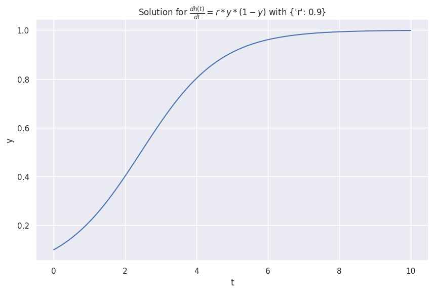
The logistic model of infectious disease is
class Infections(DiffEqn):
    def fn(self, y: float, t: np.ndarray) -> np.ndarray:
        r = self.fn_args["r"]
        dydt = r * y * (1 - y)
        return dydt

    def _formula(self):
        return r"\frac{dh(t)}{d t} = r * y * (1-y)"

infections_s = Infections(t, 0.1, r=0.9)
infections_s.plot()
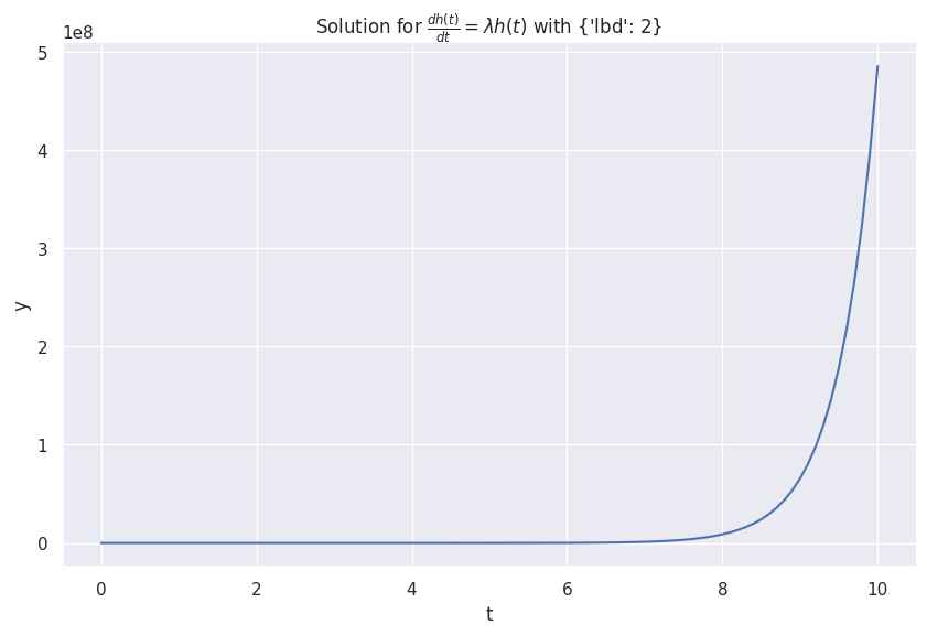
The following equation describes an exponentially growing \(h(t)\).
with \(\lambda > 0\).
class Exponential(DiffEqn):
    def fn(self, y: float, t: np.ndarray) -> np.ndarray:
        lbd = self.fn_args["lbd"]
        dydt = lbd * y

        return dydt

    def _formula(self):
        return r"\frac{dh(t)}{d t} = \lambda h(t)"

y0_exponential = 1
t = np.linspace(0, 10, 101)
lbd = 2

exponential = Exponential(t, y0_exponential, lbd=lbd)
exponential.plot()
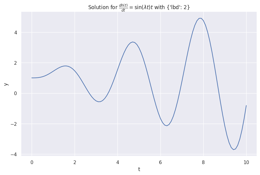
We construct an oscillatory system using sinusoid,
Naively, we expect the oscillations to be large for larger \(t\). Taking the limit \(t\to\infty\), the first order derivative \(\frac{\mathrm dy}{\mathrm d t}\to\infty\). With this limit, we expect the oscillation amplitude to be infinite.
class SinMultiplyT(DiffEqn):
    def fn(self, y: float, t: np.ndarray) -> np.ndarray:
        lbd = self.fn_args["lbd"]
        dydt = np.sin(lbd * t) * t

        return dydt

    def _formula(self):
        return r"\frac{dh(t)}{d t} = \sin(\lambda t) t"

y0_sin = 1
t = np.linspace(0, 10, 101)
lbd = 2
sin_multiply_t = SinMultiplyT(t, y0_sin, lbd=lbd)
sin_multiply_t.plot()
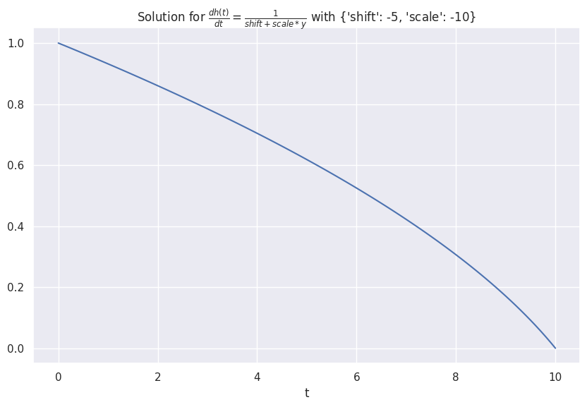
We design a system that grows according to the receprocal of its value,
class Receprocal(DiffEqn):
    def fn(self, y: float, t: np.ndarray) -> np.ndarray:
        shift = self.fn_args["shift"]
        scale = self.fn_args["scale"]
        dydt = 1/(shift + scale * y)
        return dydt

    def _formula(self):
        return r"\frac{dh(t)}{d t} = \frac{1}{shift + scale * y}"

receprocal = Receprocal(t, 1, shift=-5, scale=-10)
receprocal.plot()
Finite Difference Form of Differential Equations
Eq. \(\eqref{eq:1st-order-ode}\) can be rewritten in the finite difference form as
with \(\Delta t\) small enough.
Derivatives
The definition of the first-order derivative is $$ h'(t) = \lim_{\Delta t\to 0} \frac{h(t+\Delta t) - h(t)}{\Delta t}. $$
In a numerical computation, \(\lim\) is approached by taking a small \(\Delta t\).
If we take \(\Delta t = 1\), the equation becomes
\(\Delta t = 1\)? Rescale of Time \(t\).
As there is no absolute measure of time \(t\), we can always rescale \(t\) to \(\hat t\) so that \(\Delta t = 1\). However, for the sake of clarity, we will keep \(t\) as the time variable.
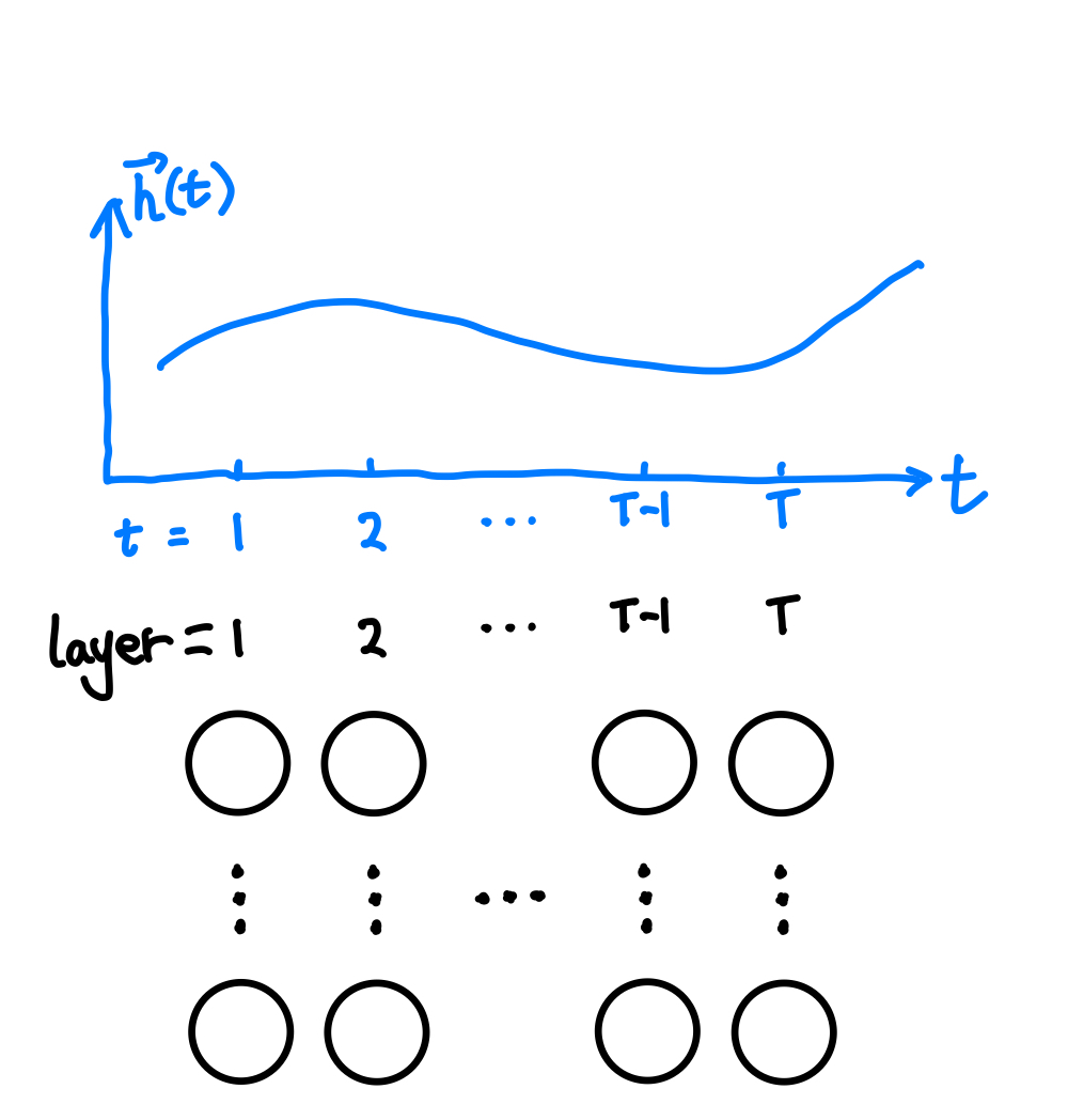
Coming back to neural networks, if \(h(t)\) represents the state of a neural network block at depth \(t\), Eq. \(\eqref{eq:1st-order-ode-finite-difference-deltat-1}\) is nothing fancy but the residual connection in ResNet2. This connection between the finite difference form of a first-order differential equation and the residual connection leads to the new family of deep neural network models called neural ode1.
In a neural ODE, we treat each layer of a neural network as a function \(h\) of depth \(t\), i.e., the state of the layer is equivalent to a function \(h(t)\). However, we are not obliged to use \(h\) as the function to directly take in the raw input and output the raw output. NeuralODE is extremely flexible and we could build latent dynamical systems to represent some intrinsic dynamics.
Solving Differential Equations
The right side of the Eq. \(\eqref{eq:1st-order-ode}\) is called the Jacobian. Given any Jacobian \(f(h(t), \theta(t), t)\), we can, at least numerically, perform integration to find out the value of \(h(t)\) at any \(t=t_N\),
In this formalism, we find out the transformed input \(h(t_0)\) by solving this differential equation. In traditional neural networks, we achieve this by stacking many layers of neural networks using skip connections.
In the original Neural ODE paper, the authors used the so-called reverse-model derivative method1.
We will not dive deep into solving differential equations in this section. Instead, we will show some applications of neural ODEs in section Time Series Forecasting with Neural ODE.
-
Chen RTQ, Rubanova Y, Bettencourt J, Duvenaud D. Neural ordinary differential equations. 2018.http://arxiv.org/abs/1806.07366. ↩↩↩
-
He K, Zhang X, Ren S, Sun J. Deep residual learning for image recognition. 2015.http://arxiv.org/abs/1512.03385. ↩