Gini Impurity

Suppose we have a dataset \(\{0,1\}^{10}\), which has 10 records and 2 possible classes of objects \(\{0,1\}\) in each record.

The first example we investigate is a pure 0 dataset.

object
0
0
0
0
0
0
0
0
0
0
0
0

For such an all-0 dataset, we would like to define its impurity as 0. Same with an all-1 dataset. For a dataset with 50% of 1 and 50% of 0, we would define its impurity as max due to the symmetries between 0 and 1.

Definition

Given a dataset \(\{0,1,...,d\}^n\), the Gini impurity is calculated as

\[ G = \sum_{i \in \{0,1,...,d\} } p(i)(1-p(i)), \]

where \(p(i)\) is the probability of a randomly picked record being class \(i\).

In the above example, we have two classes, \(\{0,1\}\). The probabilities are

\[ \begin{align} p(0) =& 1\\ p(1) =& 0 \end{align}. \]

The Gini impurity is

\[ G = p(0)(1-p(0)) + p(1)(1-p(1)) = 0+0 = 0. \]

Examples

Suppose we have another dataset with 50% of the values being 50%.

object
0
0
1
0
0
1
1
1
0
0
0
1

The Gini impurity is

\[ G = p(0)(1-p(0)) + p(1)(1-p(1)) = 0.5 * 0.5+ 0.5*0.5 = 0.5. \]

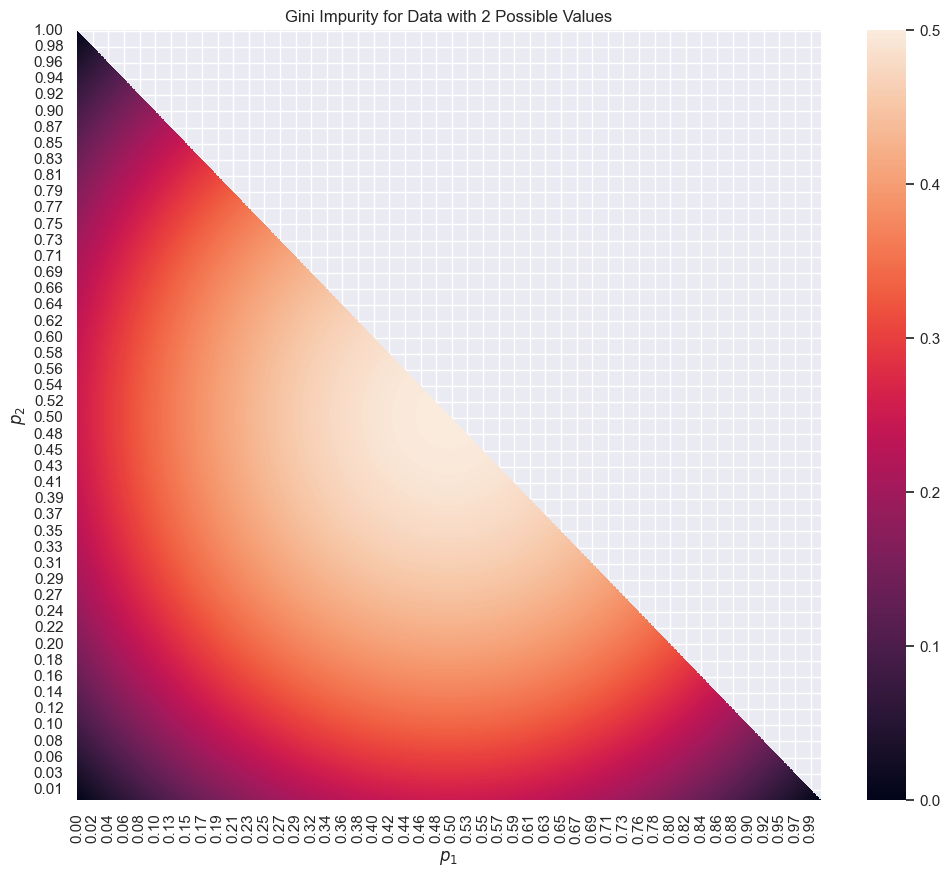
For data with two possible values \(\{0,1\}\), the maximum Gini impurity is 0.25. The following chart shows all the possible values of the Gini impurity for a two-value dataset.

The following heatmap shows the Gini impurity for data with two possible values. The color indicates the Gini impurity.

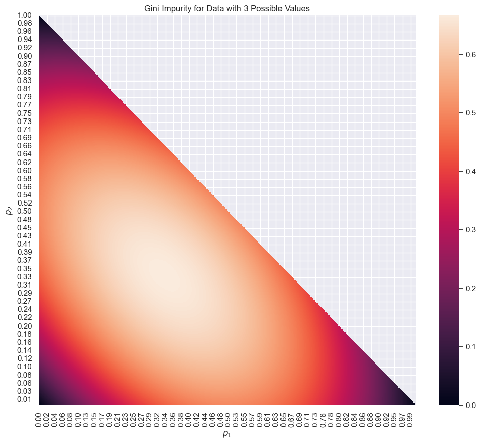
For data with three possible values, the Gini impurity is also visualized using the same chart given the condition that \(p_3 = 1 - p_1 - p_2\).

The following chart shows the Gini impurity for data with three possible values. The color indicates the Gini impurity.

---

Contributors: LM